Difference between revisions of "User:Jhurley/sandbox"

From Enviro Wiki
Jump to: navigation, search
(Thermodynamics of PFAS Accumulations on Solid Surfaces)
(Lysimeters for Measuring PFAS Concentrations in the Vadose Zone)
 
(647 intermediate revisions by the same user not shown)
Line 1: Line 1:
==Transition of Aqueous Film Forming Foam (AFFF) Fire Suppression Infrastructure Impacted by Per and Polyfluoroalkyl Substances (PFAS)==
+
==Lysimeters for Measuring PFAS Concentrations in the Vadose Zone==  
[[Perfluoroalkyl and Polyfluoroalkyl Substances (PFAS)|Per and polyfluoroalkyl substances (PFAS)]] contained in [[wikipedia:Firefighting foam |Class B aqueous film-forming foams (AFFFs)]] are known to accumulate on wetted surfaces of many fire suppression systems after decades of exposure<ref name="LangEtAl2022">Lang, J.R., McDonough, J., Guillette, T.C., Storch, P., Anderson, J., Liles, D., Prigge, R., Miles, J.A.L., Divine, C., 2022. Characterization of per- and polyfluoroalkyl substances on fire suppression system piping and optimization of removal methods. Chemosphere, 308(Part 2), 136254. [https://doi.org/10.1016/j.chemosphere.2022.136254 doi: 10.1016/j.chemosphere.2022.136254]&nbsp;&nbsp;[[Media:LangEtAl2022.pdf | Open Access Article]]</ref>. When replacement PFAS-free firefighting formulations are added to existing infrastructure, PFAS can rebound from the wetted surfaces into the new formulations at high concentrations<ref name="RossStorch2020">Ross, I., and Storch, P., 2020. Foam Transition: Is It as Simple as "Foam Out / Foam In?". The Catalyst (Journal of JOIFF, The International Organization for Industrial Emergency Services Management), Q2 Supplement, 20 pages. [[Media:Catalyst_2020_Q2_Sup.pdf | Industry Newsletter]]</ref><ref>Kappetijn, K., 2023. Replacement of fluorinated extinguishing foam: When is clean clean enough? The Catalyst (Journal of JOIFF, The International Organization for Industrial Emergency Services Management), Q1 2023, pp. 31-33. [[Media:Catalyst_2023_Q1.pdf | Industry Newsletter]]</ref>. Effective methods are needed to properly transition to PFAS-free firefighting formulations in existing fire suppression infrastructure. Considerations in the transition process may include but are not limited to locating, identifying, and evaluating existing systems and AFFF, fire engineering evaluations, system prioritization, cost/downtime analyses, sampling and analysis, evaluation of risks and hazards to human health and the environment, transportation, and disposal.
+
[[Perfluoroalkyl and Polyfluoroalkyl Substances (PFAS) | PFAS]] are frequently introduced to the environment through soil surface applications which then transport through the vadose zone to reach underlying groundwater receptors. Due to their unique properties and resulting transport and retention behaviors, PFAS in the vadose zone can be a persistent contaminant source to underlying groundwater systems. Determining the fraction of PFAS present in the mobile porewater relative to the total concentrations in soils is critical to understanding the risk posed by PFAS in vadose zone source areas. Lysimeters are instruments that have been used by agronomists and vadose zone researchers for decades to determine water flux and solute concentrations in unsaturated porewater. Lysimeters have recently been developed as a critical tool for field investigations and characterizations of PFAS impacted source zones.  
 
<div style="float:right;margin:0 0 2em 2em;">__TOC__</div>
 
<div style="float:right;margin:0 0 2em 2em;">__TOC__</div>
  
 
'''Related Article(s):'''
 
'''Related Article(s):'''
*[[Perfluoroalkyl and Polyfluoroalkyl Substances (PFAS)]]
 
*[[PFAS Sources]]
 
*[[PFAS Ex Situ Water Treatment]]
 
*[[Supercritical Water Oxidation (SCWO)]]
 
*[[PFAS Treatment by Electrical Discharge Plasma]]
 
  
'''Contributor(s):'''
+
*[[Perfluoroalkyl and Polyfluoroalkyl Substances (PFAS)]]
*Dr. Johnsie Ray Lang
+
*[[PFAS Transport and Fate]]
*Dr. Jonathan Miles
+
*[[PFAS Toxicology and Risk Assessment]]
*John Anderson
+
*[[Mass Flux and Mass Discharge]]
*Dr. Theresa Guillette
 
*[[Craig E. Divine, Ph.D., PG|Dr. Craig Divine]]
 
*[[Dr. Stephen Richardson]]
 
  
'''Key Resource(s):'''
+
'''Contributors:''' Dr. John F. Stults, Dr. Charles Schaefer
*Department of Defense (DoD) performance standard for PFAS-free firefighting formulation:  [https://media.defense.gov/2023/Jan/12/2003144157/-1/-1/1/MILITARY-SPECIFICATION-FOR-FIRE-EXTINGUISHING-AGENT-FLUORINE-FREE-FOAM-F3-LIQUID-CONCENTRATE-FOR-LAND-BASED-FRESH-WATER-APPLICATIONS.PDF Military Specification MIL-PRF-32725]<ref name="DoD2023">US Department of Defense, 2023. Performance Specification for Fire Extinguishing Agent, Fluorine-Free Foam (F3) Liquid Concentrate for Land-Based, Fresh Water Applications. Mil-Spec MIL-PRF-32725, 18 pages. [[Media: MilSpec32725.pdf | Military Specification Document]]</ref>
+
 
*Characterization of per- and polyfluoroalkyl substances on fire suppression system piping and optimization of removal methods<ref name="LangEtAl2022"/>
+
'''Key Resources:'''
 +
*Assessment of PFAS in Collocated Soil and Porewater Samples at an AFFF-Impacted Source Zone: Field-Scale Validation of Suction Lysimeters<ref name="AndersonEtAl2022"/>
 +
*PFAS Concentrations in Soil versus Soil Porewater: Mass Distributions and the Impact of Adsorption at Air-Water Interfaces<ref name="BrusseauGuo2022"/>
 +
*Using Suction Lysimeters for Determining the Potential of Per- and Polyfluoroalkyl Substances to Leach from Soil to Groundwater: A Review<ref name="CostanzaEtAl2025"/>
 +
*Use of Lysimeters for Monitoring Soil Water Balance Parameters and Nutrient Leaching<ref name="MeissnerEtAl2020"/>
 +
*PFAS Porewater Concentrations in Unsaturated Soil: Field and Laboratory Comparisons Inform on PFAS Accumulation at Air-Water Interfaces<ref name="SchaeferEtAl2024"/>
  
 
==Introduction==
 
==Introduction==
[[File:LangFig1.png | thumb |400px|Figure 1. (A) Schematic of a typical PFAS molecule demonstrating the hydrophobic fluorinated tail in green and the hydrophilic charged functional group in blue, (B) a PFAS bilayer formed with the hydrophobic tails facing inward and the charged functional groups on the outside, and (C) multiple bilayers of PFAS assembled on the wetted surfaces of fire suppression piping.]]PFAS are a class of synthetic fluorinated compounds which are highly mobile and persistent within the environment<ref>Giesy, J.P., Kannan, K., 2001. Global Distribution of Perfluorooctane Sulfonate in Wildlife. Environmental Science and Technology 35(7), pp. 1339-1342. [https://doi.org/10.1021/es001834k doi: 10.1021/es001834k]</ref>. Due to the surfactant properties of PFAS, these compounds self-assemble at any solid-liquid interface forming resilient bilayers during prolonged exposure<ref>Krafft, M.P., Riess, J.G., 2015. Selected physicochemical aspects of poly- and perfluoroalkylated substances relevant to performance, environment and sustainability-Part one. Chemosphere, 129, pp. 4-19. [https://doi.org/10.1016/j.chemosphere.2014.08.039 doi: 10.1016/j.chemosphere.2014.08.039]</ref>. Solid phase accumulation of PFAS has been proposed to be influenced by both hydrophobic and electrostatic interactions with fluorinated carbon chain length as the dominant feature influencing sorption<ref>Higgins, C.P., Luthy, R.G., 2006. Sorption of Perfluorinated Surfactants on Sediments. Environmental Science and Technology, 40(23), pp. 7251-7256. [https://doi.org/10.1021/es061000n doi: 10.1021/es061000n]</ref>. While the majority of previous research into solid phase sorption typically focused on water treatment applications or subsurface porous media<ref>Brusseau, M.L., 2018. Assessing the Potential Contributions of Additional Retention Processes to PFAS Retardation in the Subsurface. Science of the Total Environment, 613-614, pp. 176-185. [https://doi.org/10.1016/j.scitotenv.2017.09.065 doi: 10.1016/j.scitotenv.2017.09.065]&nbsp;&nbsp;[https://www.ncbi.nlm.nih.gov/pmc/articles/PMC5693257/ Open Access Manuscript]</ref>, recently PFAS accumulations have been demonstrated on the wetted surfaces of fire suppression infrastructure exposed to aqueous film forming foam (AFFF)<ref name="LangEtAl2022"/> (see Figure 1).
+
Lysimeters are devices that are placed in the subsurface above the groundwater table to monitor the movement of water through the soil<ref name="GossEhlers2009">Goss, M.J., Ehlers, W., 2009. The Role of Lysimeters in the Development of Our Understanding of Soil Water and Nutrient Dynamics in Ecosystems. Soil Use and Management, 25(3), pp. 213–223. [https://doi.org/10.1111/j.1475-2743.2009.00230.x doi: 10.1111/j.1475-2743.2009.00230.x]</ref><ref>Pütz, T., Fank, J., Flury, M., 2018. Lysimeters in Vadose Zone Research. Vadose Zone Journal, 17 (1), pp. 1-4. [https://doi.org/10.2136/vzj2018.02.0035 doi: 10.2136/vzj2018.02.0035]&nbsp; [[Media: PutzEtAl2018.pdf | Open Access Article]]</ref><ref name="CostanzaEtAl2025">Costanza, J., Clabaugh, C.D., Leibli, C., Ferreira, J., Wilkin, R.T., 2025. Using Suction Lysimeters for Determining the Potential of Per- and Polyfluoroalkyl Substances to Leach from Soil to Groundwater: A Review. Environmental Science and Technology, 59(9), pp. 4215-4229. [https://doi.org/10.1021/acs.est.4c10246 doi: 10.1021/acs.est.4c10246]</ref>. Lysimeters have historically been used in agricultural sciences for monitoring nutrient or contaminant movement, soil moisture release curves, natural drainage patterns, and dynamics of plant-water interactions<ref name="GossEhlers2009"/><ref>Bergström, L., 1990. Use of Lysimeters to Estimate Leaching of Pesticides in Agricultural Soils. Environmental Pollution, 67 (4), 325–347. [https://doi.org/10.1016/0269-7491(90)90070-S doi: 10.1016/0269-7491(90)90070-S]</ref><ref>Dabrowska, D., Rykala, W., 2021. A Review of Lysimeter Experiments Carried Out on Municipal Landfill Waste. Toxics, 9(2), Article 26. [https://doi.org/10.3390/toxics9020026 doi: 10.3390/toxics9020026]&nbsp; [[Media: Dabrowska Rykala2021.pdf | Open Access Article]]</ref><ref>Fernando, S.U., Galagedara, L., Krishnapillai, M., Cuss, C.W., 2023. Lysimeter Sampling System for Optimal Determination of Trace Elements in Soil Solutions. Water, 15(18), Article 3277. [https://doi.org/10.3390/w15183277 doi: 10.3390/w15183277]&nbsp; [[Media: FernandoEtAl2023.pdf | Open Access Article]]</ref><ref name="MeissnerEtAl2020">Meissner, R., Rupp, H., Haselow, L., 2020. Use of Lysimeters for Monitoring Soil Water Balance Parameters and Nutrient Leaching. In: Climate Change and Soil Interactions. Elsevier, pp. 171-205. [https://doi.org/10.1016/B978-0-12-818032-7.00007-2 doi: 10.1016/B978-0-12-818032-7.00007-2]</ref><ref name="RogersMcConnell1993">Rogers, R.D., McConnell, J.W. Jr., 1993. Lysimeter Literature Review, Nuclear Regulatory Commission Report Numbers: NUREG/CR--6073, EGG--2706. [https://www.osti.gov/] ID: 10183270. [https://doi.org/10.2172/10183270 doi: 10.2172/10183270]&nbsp; [[Media: RogersMcConnell1993.pdf | Open  Access Article]]</ref><ref>Sołtysiak, M., Rakoczy, M., 2019. An Overview of the Experimental Research Use of Lysimeters. Environmental and Socio-Economic Studies, 7(2), pp. 49-56. [https://doi.org/10.2478/environ-2019-0012 doi: 10.2478/environ-2019-0012]&nbsp; [[Media: SołtysiakRakoczy2019.pdf | Open Access Article]]</ref><ref name="Stannard1992">Stannard, D.I., 1992. Tensiometers—Theory, Construction, and Use. Geotechnical Testing Journal, 15(1), pp. 48-58. [https://doi.org/10.1520/GTJ10224J doi: 10.1520/GTJ10224J]</ref><ref name="WintonWeber1996">Winton, K., Weber, J.B., 1996. A Review of Field Lysimeter Studies to Describe the Environmental Fate of Pesticides. Weed Technology, 10(1), pp. 202-209. [https://doi.org/10.1017/S0890037X00045929 doi: 10.1017/S0890037X00045929]</ref>. Recently, there has been strong interest in the use of lysimeters to measure and monitor movement of per- and polyfluoroalkyl substances (PFAS) through the vadose zone<ref name="Anderson2021">Anderson, R.H., 2021. The Case for Direct Measures of Soil-to-Groundwater Contaminant Mass Discharge at AFFF-Impacted Sites. Environmental Science and Technology, 55(10), pp. 6580-6583. [https://doi.org/10.1021/acs.est.1c01543 doi: 10.1021/acs.est.1c01543]</ref><ref name="AndersonEtAl2022">Anderson, R.H., Feild, J.B., Dieffenbach-Carle, H., Elsharnouby, O., Krebs, R.K., 2022. Assessment of PFAS in Collocated Soil and Porewater Samples at an AFFF-Impacted Source Zone: Field-Scale Validation of Suction Lysimeters. Chemosphere, 308(1), Article 136247. [https://doi.org/10.1016/j.chemosphere.2022.136247 doi: 10.1016/j.chemosphere.2022.136247]</ref><ref name="SchaeferEtAl2024">Schaefer, C.E., Nguyen, D., Fang, Y., Gonda, N., Zhang, C., Shea, S., Higgins, C.P., 2024. PFAS Porewater Concentrations in Unsaturated Soil: Field and Laboratory Comparisons Inform on PFAS Accumulation at Air-Water Interfaces. Journal of Contaminant Hydrology, 264, Article 104359. [https://doi.org/10.1016/j.jconhyd.2024.104359 doi: 10.1016/j.jconhyd.2024.104359]&nbsp; [[Media: SchaeferEtAl2024.pdf | Open Access Manuscript]]</ref><ref name="SchaeferEtAl2023">Schaefer, C.E., Lavorgna, G.M., Lippincott, D.R., Nguyen, D., Schaum, A., Higgins, C.P., Field, J., 2023. Leaching of Perfluoroalkyl Acids During Unsaturated Zone Flushing at a Field Site Impacted with Aqueous Film Forming Foam. Environmental Science and Technology, 57(5), pp. 1940-1948. [https://doi.org/10.1021/acs.est.2c06903 doi: 10.1021/acs.est.2c06903]</ref><ref name="SchaeferEtAl2022">Schaefer, C.E., Lavorgna, G.M., Lippincott, D.R., Nguyen, D., Christie, E., Shea, S., O’Hare, S., Lemes, M.C.S., Higgins, C.P., Field, J., 2022. A Field Study to Assess the Role of Air-Water Interfacial Sorption on PFAS Leaching in an AFFF Source Area. Journal of Contaminant Hydrology, 248, Article 104001. [https://doi.org/10.1016/j.jconhyd.2022.104001 doi: 10.1016/j.jconhyd.2022.104001]&nbsp; [[Media: SchaeferEtAl2022.pdf | Open Access Manuscript]]</ref><ref name="QuinnanEtAl2021">Quinnan, J., Rossi, M., Curry, P., Lupo, M., Miller, M., Korb, H., Orth, C., Hasbrouck, K., 2021. Application of PFAS-Mobile Lab to Support Adaptive Characterization and Flux-Based Conceptual Site Models at AFFF Releases. Remediation, 31(3), pp. 7-26. [https://doi.org/10.1002/rem.21680 doi: 10.1002/rem.21680]</ref>. PFAS are frequently introduced to the environment through land surface application and have been found to be strongly retained within the upper 5 feet of soil<ref name="BrusseauEtAl2020">Brusseau, M.L., Anderson, R.H., Guo, B., 2020. PFAS Concentrations in Soils: Background Levels versus Contaminated Sites. Science of The Total Environment, 740, Article 140017. [https://doi.org/10.1016/j.scitotenv.2020.140017 doi: 10.1016/j.scitotenv.2020.140017]</ref><ref name="BiglerEtAl2024">Bigler, M.C., Brusseau, M.L., Guo, B., Jones, S.L., Pritchard, J.C., Higgins, C.P., Hatton, J., 2024. High-Resolution Depth-Discrete Analysis of PFAS Distribution and Leaching for a Vadose-Zone Source at an AFFF-Impacted Site. Environmental Science and Technology, 58(22), pp. 9863-9874. [https://doi.org/10.1021/acs.est.4c01615 doi: 10.1021/acs.est.4c01615]</ref>. PFAS recalcitrance in the vadose zone means that environmental program managers and consultants need a cost-effective way of monitoring concentration conditions within the vadose zone. Repeated soil sampling and extraction processes are time consuming and only give a representative concentration of total PFAS in the matrix<ref name="NickersonEtAl2020">Nickerson, A., Maizel, A.C., Kulkarni, P.R., Adamson, D.T., Kornuc, J. J., Higgins, C.P., 2020. Enhanced Extraction of AFFF-Associated PFASs from Source Zone Soils. Environmental Science and Technology, 54(8), pp. 4952-4962. [https://doi.org/10.1021/acs.est.0c00792 doi: 10.1021/acs.est.0c00792]</ref>, not what is readily transportable in mobile porewater<ref name="SchaeferEtAl2023"/><ref name="StultsEtAl2024">Stults, J.F., Schaefer, C.E., Fang, Y., Devon, J., Nguyen, D., Real, I., Hao, S., Guelfo, J.L., 2024. Air-Water Interfacial Collapse and Rate-Limited Solid Desorption Control Perfluoroalkyl Acid Leaching from the Vadose Zone. Journal of Contaminant Hydrology, 265, Article 104382. [https://doi.org/10.1016/j.jconhyd.2024.104382 doi: 10.1016/j.jconhyd.2024.104382]&nbsp; [[Media: StultsEtAl2024.pdf | Open Access Manuscript]]</ref><ref name="StultsEtAl2023">Stults, J.F., Choi, Y.J., Rockwell, C., Schaefer, C.E., Nguyen, D.D., Knappe, D.R.U., Illangasekare, T.H., Higgins, C.P., 2023. Predicting Concentration- and Ionic-Strength-Dependent Air–Water Interfacial Partitioning Parameters of PFASs Using Quantitative Structure–Property Relationships (QSPRs). Environmental Science and Technology, 57(13), pp. 5203-5215. [https://doi.org/10.1021/acs.est.2c07316 doi: 10.1021/acs.est.2c07316]</ref><ref name="BrusseauGuo2022">Brusseau, M.L., Guo, B., 2022. PFAS Concentrations in Soil versus Soil Porewater: Mass Distributions and the Impact of Adsorption at Air-Water Interfaces. Chemosphere, 302, Article 134938. [https://doi.org/10.1016/j.chemosphere.2022.134938 doi: 10.1016/j.chemosphere.2022.134938]&nbsp; [[Media: BrusseauGuo2022.pdf | Open Access Manuscript]]</ref>. Fortunately, lysimeters have been found to be a viable option for monitoring the concentration of PFAS in the mobile porewater phase in the vadose zone<ref name="Anderson2021"/><ref name="AndersonEtAl2022"/>. Note that while some lysimeters, known as weighing lysimeters, can directly measure water flux, the most commonly utilized lysimeters in PFAS investigations only provide measurements of porewater concentrations.
     
 
Fire suppression systems with potential PFAS impacts include fire fighting vehicles that carried AFFF and fixed suppression systems in buildings containing large amounts of flammable materials such as aircraft hangars (Figure 2). PFAS residue on the wetted surfaces of existing infrastructure can rebound into replacement PFAS-free firefighting formulations if not removed during the transition process<ref name="RossStorch2020"/>. Simple surface rinsing with water and low-pressure washing has been proven to be inefficient for removal of surface bound PFAS from piping and tanks that contained fluorinated AFFF<ref name="RossStorch2020"/>
 
[[File:LangFig2.png | thumb|left|600px|Figure 2. Fixed fire suppression system for an aircraft hangar, with storage tank on left and distribution piping on right.]]


In&nbsp;addition&nbsp;to&nbsp;proper methods for system cleaning to remove residual PFAS, transition to PFAS-free foam may also include consideration of compliance with state and federal regulations, selection of the replacement PFAS free firefighting formulation, a cost benefit analysis for replacement of the system components versus cleaning, and PFAS verification testing. Foam transition should be completed in a manner which minimizes the volume of waste generated as well as preventing any PFAS release into the environment.


==PFAS Assembly on Solid Surfaces==
 
The self-assembly of [[Wikipedia: Amphiphile | amphiphilic]] molecules into supramolecular bilayers is a result of their structure and how it interacts with the bulk water of a solution. Single chain hydrocarbon based amphiphiles can form [[Wikipedia: Micelle | micelles]] under relatively dilute aqueous concentrations, however for hydrocarbon based surfactants the formation of more complex organized system such as [[Wikipedia: Vesicle (biology and chemistry) | vesicles]] is rarely seen, requiring double chain amphiphiles such as phospholipids. Associations of single chain cationic and anionic hydrocarbon based amphiphiles into stable supramolecular structures such as vesicles has however been demonstrated<ref>Fukuda, H., Kawata, K., Okuda, H., 1990. Bilayer-Forming Ion-Pair Amphiphiles from Single-Chain Surfactants. Journal of the American Chemical Society, 112(4), pp. 1635-1637. [https://doi.org/10.1021/ja00160a057 doi: 10.1021/ja00160a057]</ref>, with the ion pairing of the polar head groups mimicking the a double tail situation. The behavior of single chain fluorosurfactant amphiphiles has been demonstrated to be significantly different from similar hydrocarbon based analogues. Not only are [[Wikipedia: Critical micelle concentration | critical micelle concentrations (CMC)]] of fluorosurfactants typically two orders of magnitude lower than corresponding hydrocarbon surfactants but self-assembly can occur even when fluorosurfactants are dispersed at low concentrations significantly below the CMC in water and other solvents<ref name="Krafft2006">Krafft, M.P., 2006. Highly fluorinated compounds induce phase separation in, and nanostructuration of liquid media. Possible impact on, and use in chemical reactivity control. Journal of Polymer Science Part A: Polymer Chemistry, 44(14), pp. 4251-4258. [https://doi.org/10.1002/pola.21508 doi: 10.1002/pola.21508]&nbsp;&nbsp;[[Media:Krafft2006.pdf | Open Access Article]]</ref>. The assembly of fluorinated amphiphiles structurally similar to those found in AFFF have been shown to readily form stable, complex structures including vesicles, fibers, and globules at concentrations as low as 0.5% w/v in contrast to their hydrocarbon analogues which remained fluid at 30% w/v<ref>Krafft, M.P., Guilieri, F., Riess, J.G., 1993. Can Single-Chain Perfluoroalkylated Amphiphiles Alone form Vesicles and Other Organized Supramolecular Systems? Angewandte Chemie International Edition in English, 32(5), pp. 741-743. [https://doi.org/10.1002/anie.199307411 doi: 10.1002/anie.199307411]</ref><ref name="KrafftEtAl_1994">Krafft, M.P., Guilieri, F., Riess, J.G., 1994. Supramolecular assemblies from single chain perfluoroalkylated phosphorylated amphiphiles. Colloids and Surfaces A: Physicochemical and Engineering Aspects, 84(1), pp. 113-119. [https://doi.org/10.1016/0927-7757(93)02681-4 doi: 10.1016/0927-7757(93)02681-4]</ref>.


Krafft found that fluorinated amphiphiles formed bilayer membranes with phospholipids, and that the resulting vesicles were more stable than those made of phospholipids alone<ref name="KrafftEtAl_1998">Krafft, M.P., Riess, J.G., 1998. Highly Fluorinated Amphiphiles and Collodial Systems, and their Applications in the Biomedical Field. A Contribution. Biochimie, 80(5-6), pp. 489-514. [https://doi.org/10.1016/S0300-9084(00)80016-4 doi: 10.1016/S0300-9084(00)80016-4]</ref>. The similarities in amphiphilic properties between phospholipids and the hydrocarbon-based surfactants in AFFF suggests that bilayer vesicles may form between these and the fluorosurfactants also present in the concentrate. Krafft demonstrated that both the permeability of resulting mixed vesicles and their propensity to fuse with each other at increasing ionic strength was reduced as a result of the creation of an inert hydrophobic and lipophobic film within the membrane, and also suggested that the fluorinated amphiphiles increased [[Wikipedia: van der Waals force | van der Waals interactions]] in the hydrocarbon region<ref name="KrafftEtAl_1998"/>. Thus this low permeability may allow vesicles formed by the surfactants present in AFFF to act as long term repositories of PFAS not only as part of the bilayer itself but also solvated within the vesicle. This prediction is supported by the observation that supramolecular structures formed from single chain fluorinated amphiphiles have been demonstrated to be stable at elevated temperature (15 min at 121&deg;C) and have been shown to be stable over periods of months, even increasing in size over time when stored at environmentally relevant temperatures<ref name="KrafftEtAl_1994"/>.


Formation of complex structures at relatively low solute concentrations requires the monomer molecules to be well ordered to maintain tight packing in the supramolecular structure<ref>Ringsdorf, H., Schlarb, B., Venzmer, J., 1988. Molecular Architecture and Function of Polymeric Oriented Systems: Models for the Study of Organization, Surface Recognition, and Dynamics of Biomembranes. Angewandte Chemie International Edition in English, 27(1), pp. 113-158. [https://doi.org/10.1002/anie.198801131 doi: 10.1002/anie.198801131]</ref>. This order results from electrostatic forces, hydrogen bonding, and in the case of fluorinated amphiphiles, hydrophobic interactions. The geometry of the amphiphile also potentially contributes to the type of supramolecular aggregation<ref>Israelachvili, J.N., Mitchell, D.J., Ninham, B.W., 1976. Theory of Self-Assembly of Hydrocarbon Amphiphiles into Micelles and Bilayers. Journal of the Chemical Society, Faraday Transactions 2: Molecular and Chemical Physics, 72, pp. 1525-1568. [https://doi.org/10.1039/F29767201525 doi: 10.1039/F29767201525]</ref>. Surfactants which adopt a conical shape (such as a typical hydrocarbon based surfactant with a large polar head group and a single alkyl chain as a tail) tend to form micelles more easily. Increasing the bulk of the tail makes the surfactant more cylindrically shaped which makes assembly into bilayers more likely.  


Perfluoroalkyl chains are significantly more bulky than their hydrocarbon based analogues both in cross sectional area (28-30 Å<sup>2</sup> versus 20 Å<sup>2</sup>, respectively) and mean volume (CF<sub>2</sub> and CF<sub>3</sub> estimated as 38 Å<sup>3</sup> and 92 Å<sup>3</sup> compared to 27 Å<sup>3</sup> and 54 Å<sup>3</sup> for CH<sub>2</sub> and CH<sub>3</sub>)<ref name="KrafftEtAl_1998"/><ref name="Krafft2006"/>. Structural studies on linear PFOS have shown that the molecule adopts an unusual helical structure<ref>Erkoç, Ş., Erkoç, F., 2001. Structural and electronic properties of PFOS and LiPFOS. Journal of Molecular Structure: THEOCHEM, 549(3), pp. 289-293. [https://doi.org/10.1016/S0166-1280(01)00553-X doi:10.1016/S0166-1280(01)00553-X]</ref><ref name="TorresEtAl2009">Torres, F.J., Ochoa-Herrera, V., Blowers, P., Sierra-Alvarez, R., 2009. Ab initio study of the structural, electronic, and thermodynamic properties of linear perfluorooctane sulfonate (PFOS) and its branched isomers. Chemosphere 76(8), pp. 1143-1149. [https://doi.org/10.1016/j.chemosphere.2009.04.009 doi: 10.1016/j.chemosphere.2009.04.009]</ref> in aqueous and solvent phases to alleviate steric hindrance. This arrangement results from the carbon chain starting in the planar all anti conformation and then successively twisting all the CC-CC dihedrals by 15&deg;-20&deg; in the same direction<ref>Abbandonato, G., Catalano, D., Marini, A., 2010. Aggregation of Perfluoroctanoate Salts Studied by <sup>19</sup>F NMR and DFT Calculations: Counterion Complexation, Poly(ethylene glycol) Addition, and Conformational Effects. Langmuir 26(22), pp. 16762-16770. [https://doi.org/10.1021/la102578k  doi: 10.1021/la102578k].</ref>. The conformation also minimizes the electrostatic repulsion between fluorine atoms bonded to the same side of the carbon backbone by maximizing the interatomic distances between them<ref name="TorresEtAl2009"/>.


A consequence of the helical structure is that there is limited carbon-carbon bond rotation within the perfluoroalkyl chain giving them increased rigidity compared to alkyl chains<ref>Barton, S.W., Goudot, A., Bouloussa, O., Rondelez, F., Lin, B., Novak, F., Acero, A., Rice, S., 1992. Structural transitions in a monolayer of fluorinated amphiphile molecules. The Journal of Chemical Physics, 96(2), pp. 1343-1351. [https://doi.org/10.1063/1.462170 doi: 10.1063/1.462170]</ref>. The bulkiness of the perfluoroalkyl chain confers a cylindrical shape on the fluorosurfactant amphiphile and therefore favors the formation of bilayers and vesicles the aggregation of which is further assisted by the rigidity of the molecules which allow close packing in the supramolecular structure. Fluorosurfactants therefore cannot be regarded as more hydrophobic analogues of hydrogenated surfactants. Their self-assembly behavior is characterized by a strong tendency to form vesicles and lamellar phases rather than micelles, due to the bulkiness and rigidity of the perfluoroalkyl chain that tends to decrease the curvature of the aggregates they form in solution<ref>Barton, C.A., Butler, L.E., Zarzecki, C.J., Flaherty, J., Kaiser, M., 2006. Characterizing Perfluorooctanoate in Ambient Air near the Fence Line of a Manufacturing Facility: Comparing Modeled and Monitored Values. Journal of the Air and Waste Management Association, 56, pp. 48-55. [https://doi.org/10.1080/10473289.2006.10464429 doi: 10.1080/10473289.2006.10464429]&nbsp;&nbsp;[https://www.tandfonline.com/doi/epdf/10.1080/10473289.2006.10464429?needAccess=true Open Access Article]</ref>. The larger tail cross section of fluorinated compared to hydrogenated amphiphiles tends to favor the formation of aggregates with lesser surface curvature, therefore rather than micelles they form bilayer membranes, vesicles, tubules and fibers<ref>Krafft, M.P., Guilieri, F., Riess, J.G., 1993. Can Single-Chain Perfluoroalkylated Amphiphiles Alone form Vesicles and Other Organized Supramolecular Systems? Angewandte Chemie International Edition in English, 32(5), pp. 741-743. [https://doi.org/10.1002/anie.199307411 doi: 10.1002/anie.199307411]</ref><ref>Furuya, H., Moroi, Y., Kaibara, K., 1996. Solid and Solution Properties of Alkylammonium Perfluorocarboxylates. The Journal of Physical Chemistry, 100(43), pp. 17249-17254.  [https://doi.org/10.1021/jp9612801 doi: 10.1021/jp9612801]</ref><ref>Giulieri, F., Krafft, M.P., 1996. Self-organization of single-chain fluorinated amphiphiles with fluorinated alcohols. Thin Solid Films, 284-285, pp. 195-199. [https://doi.org/10.1016/S0040-6090(95)08304-9 doi: 10.1016/S0040-6090(95)08304-9]</ref><ref>Gladysz, J.A., Curran, D.P., Horvath, I.T., 2004. Handbook of Fluorous Chemistry. WILEY-VCH Verlag GmbH & Co. KGaA,, Weinheim, Germany. ISBN: 3-527-30617-X</ref>. Rojas ''et al.'' (2002) demonstrated that perfluorooctyl sulphonamide formed a contiguous bilayer at 50 mg/L with self-assembled aggregates present at concentrations as low as 10 mg/L<ref name="RojasEtAl2002">Rojas, O.J., Macakova, L., Blomberg, E., Emmer, A., and Claesson, P.M., 2002. Fluorosurfactant Self-Assembly at Solid/Liquid Interfaces. Langmuir, 18(21), pp. 8085-8095. [https://doi.org/10.1021/la025989c doi: 10.1021/la025989c]</ref>.     


==Thermodynamics of PFAS Accumulations on Solid Surfaces==
 
The thermodynamics of formation of amphiphiles into supramolecular species requires consideration of both hydrophobic and hydrophilic interactions resulting from the amphoteric nature of the molecule. The hydrophilic portions of the molecule are driven to maximize their solvation interaction with as many water molecules as possible, whereas the hydrophobic portions of the molecule are driven to aggregate together thus minimizing interaction with the bulk water. Both of these processes change the enthalpy and entropy of the system.


In aqueous solution, the hydrophilic portions of an amphiphile form hydrogen bonds (4 - 120 kJ/mol) and van der Waals interactions (<5 kJ/mol) with water molecules and surfaces, and electrostatic interactions (5 – 300 kJ/mol) can also occur where the amphiphile is ionic<ref name="LombardoEtAl2015">Lombardo, D., Kiselev, M.A., Magazù, S., Calandra, P., 2015. Amphiphiles Self-Assembly: Basic Concepts and Future Perspectives of Supramolecular Approaches. Advances in Condensed Matter Physics, vol. 2015, article ID 151683, 22 pages. [https://doi.org/10.1155/2015/151683 doi: 10.1155/2015/151683]&nbsp;&nbsp;[[Media: LombardoEtAl2015.pdf | Open Access Article]]</ref>. These interactions, although weak compared to intramolecular covalent bonds within a molecule are energetically favorable and increase the enthalpy of the combined solute-solvent system. Thus, the hydrophilic portion of an amphiphile will look to maximize enthalpic gain through hydrogen bond interactions with the bulk water.


The hydrophobic portion of an amphiphile cannot form hydrogen bonds with the bulk solution, and its presence disrupts the hydrogen bond interactions between individual water molecules within the bulk water matrix. This disruption lowers the entropy of the system by reducing the degrees of translational rotational freedom available to the bulk water. The second law of thermodynamics dictates that a system will arrange itself to maximize its entropy. With hydrophobic species this can be achieved by their spontaneous aggregation, as the reduction in solution entropy of the aggregated system is less than that which would occur if the component parts were solvated individually. These hydrophobic and hydrophilic interactions are weak, and the individual entropy gain per amphiphile upon aggregation is very small. However, taken together the overall effect on the entropy of the aggregate is sufficient to maintain it in solution, and moreover these interactions make the aggregates resistant to minor perturbations while retaining the reversibility of the self-assembled structure<ref name="LombardoEtAl2015"/>.


==Regulatory Drivers for Transition to PFAS Free Firefighting Formulations==
 
Regulations restricting the use and release of PFAS are being proposed and promulgated worldwide, with several enacted regulations addressing the use of aqueous film forming foams (AFFF) containing PFAS


Discharges of contaminated groundwater to surface water bodies threaten ecosystems and degrade the quality of surface water resources. Subsurface heterogeneity associated with the geological setting and stratigraphy often results in such discharges occurring as localized zones (or seeps) of contaminated groundwater. Traditional methods for investigating GWSWE include [https://books.gw-project.org/groundwater-surface-water-exchange/chapter/seepage-meters/#:~:text=Seepage%20meters%20measure%20the%20flux,that%20it%20isolates%20water%20exchange. seepage meters]<ref>Rosenberry, D. O., Duque, C., and Lee, D. R., 2020. History and Evolution of Seepage Meters for Quantifying Flow between Groundwater and Surface Water: Part 1 – Freshwater Settings. Earth-Science Reviews, 204(103167). [https://doi.org/10.1016/j.earscirev.2020.103167 doi: 10.1016/j.earscirev.2020.103167].</ref><ref>Duque, C., Russoniello, C. J., and Rosenberry, D. O., 2020. History and Evolution of Seepage Meters for Quantifying Flow between Groundwater and Surface Water: Part 2 – Marine Settings and Submarine Groundwater Discharge. Earth-Science Reviews, 204 ( 103168). [https://doi.org/10.1016/j.earscirev.2020.103168 doi: 10.1016/j.earscirev.2020.103168].</ref>, which directly quantify the volume flux crossing the bed of a surface water body (i.e, a  lake, river or wetland) and point probes that locally measure key water quality parameters (e.g., temperature, pore water velocity, specific conductance, dissolved oxygen, pH). Seepage meters provide direct estimates of seepage fluxes between groundwater and surface- water but are time consuming and can be difficult to deploy in high energy surface water environments and along armored bed sediments. Manual seepage meters rely on quantifying volume changes in a bag of water that is hydraulically connected to the bed. Although automated seepage meters such as the [https://clu-in.org/programs/21m2/navytools/gsw/#ultraseep Ultraseep system] have been developed, they are generally not suitable for long term deployment (weeks to months). The US Navy has developed the [https://clu-in.org/programs/21m2/navytools/gsw/#trident Trident probe] for more rapid (relative to seepage meters) sampling, whereby the probe is inserted into the bed and point-in-time pore water quality and sediment parameters are directly recorded (note that the Trident probe does not measure a seepage flux). Such direct probe-based measurements are still relatively time consuming to acquire, particularly when reconnaissance information is required over large areas to determine the location of discrete seeps for further, more quantitative analysis.


Over the last few decades, a broader toolbox of hydrogeophysical technologies has been developed to rapidly and non-invasively evaluate zones of GWSWE in a variety of surface water settings, spanning from freshwater bodies to saline coastal environments. Many of these technologies are currently being deployed under a Department of Defense Environmental Security Technology Certification Program ([https://serdp-estcp.mil/ ESTCP]) project ([https://serdp-estcp.mil/projects/details/e4a12396-4b56-4318-b9e5-143c3011b8ff ER21-5237]) to demonstrate the value of the toolbox to remedial program managers (RPMs) dealing with the challenge of characterizing surface water contamination via groundwater from facilities proximal to surface water bodies. This article summarizes these technologies and provides references to key resources, mostly provided by the [https://www.usgs.gov/mission-areas/water-resources Water Resources Mission Area] of the United States Geological Survey that describe the technologies in further detail.


==Hydrogeophysical Technologies for Understanding Groundwater-Surface Water Interactions==
 
[[Wikipedia: Hydrogeophysics |Hydrogeophysical technologies]] exploit contrasts in the physical properties between groundwater and surface water to detect and monitor zones of pronounced GWSWE. The two most valuable properties to measure are temperature and electrical conductivity. Temperature has been used for decades as an indicator of groundwater-surface water exchange<ref>Constantz, J., 2008.  Heat as a Tracer to Determine Streambed Water Exchanges. Water Resources Research, 44 (4).[https://doi.org/https://doi.org/10.1029/2008WR006996 doi: 10.1029/2008WR006996].[https://agupubs.onlinelibrary.wiley.com/doi/epdf/10.1029/2008WR006996  Open Access Article]</ref> with early uses including pushing a thermistor into the bed of a surface water body to assess zones of surface water downwelling and groundwater upwelling. Today, a variety of novel technologies that measure temperature over a wide range of spatial and temporal scales are being used to investigate GWSWE. The evaluation of electrical conductivity measurements using point probes and geophysical imaging is also well-established. However, new technologies are now available to exploit electrical conductivity contrasts from GWSWE occurring over a range of spatial and temporal scales.


===Temperature-Based Technologies===
 
Several temperature-based GWSWE methodologies exploit the gradient in temperature between surface water and groundwater that exist during certain times of day or seasons of the year. The thermal insulation provided by the Earth’s land surface means that groundwater is warmer than surface water in winter months, but colder than surface water in summer months away from the equator. Therefore, in temperate climates, localized (or ‘preferential’) groundwater discharge into surface water bodies is often observed as cold temperature anomalies in the summer and warm temperature anomalies in the winter. However, there are times of the year such as fall and spring when contrasts in the temperature between groundwater and surface water will be minimal, or even undetectable. These seasonal-driven points in time correspond to the switch in the polarity of the temperature contrast between groundwater and surface water. Consequently, SW to GW gradient temperature-based methods are most effective when deployed at times of the year when the temperature contrasts between groundwater and surface water are greatest. Other time-series temperature monitoring methods depend more on natural daily signals measured at the bed interface and in bed sediments, and those signals may exist year round except where strongly muted by ice cover or surface water stratification. A variety of sensing technologies now exist within the GWSWE toolbox, from techniques that rapidly characterize temperature contrasts over large areas, down to powerful monitoring methods that can continuously quantify GWSWE fluxes at discrete locations identified as hotspots.


====Characterization Methods====
 
The primary use of the characterization methods is to rapidly determine precise locations of groundwater upwelling over large areas in order to pinpoint locations for subsequent ground-based observations. A common limitation of these methods is that they can only sense groundwater fluxes into surface water. Methods applied at the water surface and in the surface water column generally cannot detect localized regions of surface water transfer to groundwater, for which temperature measurements collected within the bed sediments are needed. This is a more challenging characterization task that may, in the right conditions, be addressed using electrical conductivity-based methods described later in this article.


=====''Unmanned Aerial Vehicle Infrared (UAV-IR)''=====
 
[[File:IeryFig1.png | thumb |600px|Figure 1. UAV IR orthomosaics with estimated scale of (a) a wetland in winter (modified from Briggs et al.<ref>Briggs, M. A., Jackson, K. E., Liu, F., Moore, E. M., Bisson, A., Helton, A. M., 2022. Exploring Local Riverbank Sediment Controls on the Occurrence of Preferential Groundwater Discharge Points. Water, 14(1). [https://doi.org/10.3390/w14010011 doi: 10.3390/w14010011]&nbsp;&nbsp;[https://www.mdpi.com/2073-4441/14/1/11 Open Access Article].</ref>) and (b) a mountain stream in summer (modified from Briggs et al.<ref>Briggs, M. A., Wang, C., Day-Lewis, F. D., Williams, K. H., Dong, W., Lane, J. W., 2019. Return Flows from Beaver Ponds Enhance Floodplain-to-River Metals Exchange in Alluvial Mountain Catchments. Science of the Total Environment, 685, pp. 357–369. [https://doi.org/10.1016/j.scitotenv.2019.05.371 doi: 10.1016/j.scitotenv.2019.05.371].&nbsp;&nbsp;[https://pdf.sciencedirectassets.com/271800/1-s2.0-S0048969719X00273/1-s2.0-S0048969719324246/am.pdf?X-Amz-Security-Token=IQoJb3JpZ2luX2VjEE0aCXVzLWVhc3QtMSJGMEQCIBY8ykhAP941wHO1NKj8EmXG3btdpgX6HaUV9zAo0PCMAiACRjzV0D2lbFFwnhUzEqBupGsgX6DkK62ZIEvb%2B0irbiq8BQj2%2F%2F%2F%2F%2F%2F%2F%2F%2F%2F8BEAUaDDA1OTAwMzU0Njg2NSIMPmS2kZBwKKMGD%2F6GKpAFaY6lOuHO%2B1RkV%2FL6NkK74dL6YJculUqyZJn9s09njF1L%2Bb4LgjH%2FbawysWGvGeuH%2FQtSgwqFM90MQ4grDiDQPHUjSEDNVuN2II%2BqPK4oqkjqxwTmC2AObe%2FMY1c45L2nshYodZwtROh6Hl8Jp4B4HoDPE9wx1fEw7DGmB%2Bj70q5PG7%2FUUo3rLl6BCMT%2FWKFGfZSaOmaD5nweVaTRBUbgSVIcmCQKshE28TkHFpmwY58YNO0GjaKHXMsBNciZ2DvIPAHMyA1iymB7UFcoBRDicZJUDZvvnJNGj1bTX9tEQ49yil7IWD22hKPHL5nSogssocX5rRXiIglVT%2BAzHsMMyxfVxfFGBsmmSGAVG9FAeRPgx1T%2FIOqNo%2FOuyV9G%2BVSt5boUg4HBaZSvW5JNkL5bFpaMlrUTpMF%2F6Bbq3Q6EsiZMaFF0JOS3rvX5dkDlfu7OzJDBuRBszYoq%2B4%2FLQGJypfmarz8ZHEzi3Qw85nYbT68UGNa%2BZ9lZQG%2B47mF6Nj11%2F%2Fu%2FDTZD1p4r9nskTevwkRE%2BL7q3OSbqFj4YvN6qsMBLb%2FM7K2xSmaots0YGisZ09fVJBetJ1ILZpN5wCbS%2F77uFeQoxYXGIwz84wyqSueP7qcj3BQ%2FMkZRbmVpokj3vtESlfHvcZV2Ntu95JM9hetE9F5azaZ%2F%2Fm3WTE2mgW48FCbFI09p%2F7%2FSJyEWl54lNG7%2F2y0AayedFUs75otJauCpNJtr2pF4sbAGfgiagA2%2BzeDatKnI7MDhMD0R27wvaVwEup6vkLmTaJh4P8bGFd01Fwj96gZIKESW6HfwGXMBMj%2FoJn3CYpcfVelPmDr6jTeSJapUJoWE8gQVFjWuISuD4PdHYtbiSBL%2Fjn5jPvGMwvrqrrQY6sgEtK%2Fo3hSElpY%2Be20Xj4eNAJ%2BFmkb5nASAJvtygtnSdoc%2FBHMv4U3Je92nbunzwAwXaVCZ8FBK1%2F2cmq3sYLNOyPEJrCNqAo0Lgf137RvhaJb7erYXXfL7UCz1hePrG3I3bgKkBRN5PD%2FSlu%2BSSEimoEn4kCyxoaNYI9QvymaTlHZJM0ueXCYprlRfMneJXxnEVyC3qlMsTMtcL%2B45koHZeeTQJUMXWJB%2BYQxNDmNM3ZHH4&X-Amz-Algorithm=AWS4-HMAC-SHA256&X-Amz-Date=20240119T205045Z&X-Amz-SignedHeaders=host&X-Amz-Expires=300&X-Amz-Credential=ASIAQ3PHCVTYV2JHRO6K%2F20240119%2Fus-east-1%2Fs3%2Faws4_request&X-Amz-Signature=3befd4efcf96517aad4e02a2d76e82cd278f02be8a60a5136a4981889df64f00&hash=c0f70e64bfdb70375c685714475b258099c0d0b19a2a7a556e77182cc6cfac9c&host=68042c943591013ac2b2430a89b270f6af2c76d8dfd086a07176afe7c76c2c61&pii=S0048969719324246&tid=pdf-5d6462f0-c794-4158-b89d-2a1f5b96a226&sid=8b33666922432845420b6d75b151281148eegxrqa&type=client Open Access Manuscript]</ref>) that both capture multiscale groundwater discharge processes. Figure reproduced from Mangel et al.<ref>Mangel, A. R., Dawson, C. B., Rey, D. M., Briggs, M. A., 2022. Drone Applications in Hydrogeophysics: Recent Examples and a Vision for the Future. The Leading Edge, 41 (8), pp. 540–547. [https://doi.org/10.1190/tle41080540.1 doi: 10.1190/tle41080540].</ref>]]
 
[[Wikipedia: Unmanned aerial vehicle | Unmanned aerial vehicles (UAVs)]] equipped with thermal infrared (IR) cameras can provide a very powerful tool for rapidly determining zones of pronounced upwelling of groundwater to surface water. Large areas of can be covered with high spatial resolution. The information obtained can be used to rapidly define locations of focused groundwater upwelling and prioritize these for more intensive surface-based observations (Figure 1). As with all thermal methods, flights must be performed when adequate contrasts in temperature between surface water and groundwater are expected to exist. Not just time of year but, because of the effect of the diurnal temperature signal on surface water bodies, time of day might need to be considered in order to maximize the chance of success. Calibration of UAV-IR camera measurements against simultaneously acquired direct measurements of temperature is recommended to optimize the value of these datasets. UAV-IR methods will not work in all situations. One major limitation of the technology is that the temperature expression of groundwater upwelling must be manifested at the surface of the surface water body. Consequently, the technology will not detect relatively small discharges occurring beneath a relatively deep surface water layer, and thermal imaging over the water surface can be complicated by thermal IR reflection. The chances of success with UAV-IR will be strongest in regions of  exposed banks or shallow water where there are no strong currents causing mixing (and thus dilution) of the upwelling groundwater temperature signals. UAV-IR methods will therefore likely be most successful close to shorelines of lakes/ponds, over shallow, low flow streams and rivers and in wetland environments. UAV-IR methods require a licensed pilot, and restrictions on the use of airspace may limit the application of this technology.


=====''Handheld Thermal Infrared (TIR) Cameras''=====
 
[[File:IeryFig2.png | thumb|left |600px|Figure 2. (a) A TIR camera set up to image groundwater discharges to surface water (b) TIR data inset on a visible light photograph. Cooler (blue) bank seepage groundwater is discharging into warmer (red) stream water (temperature scale in degrees). Both photographs courtesy of Martin Briggs USGS.]]
 
Hand-held thermal infrared (TIR) cameras are powerful tools for visual identification of localized seeps of upwelling groundwater. TIR cameras may be used to follow up on UAV-IR surveys to better characterize local seeps identified from the air using UAV-IR. Alternatively, a TIR camera is a valuable tool when performing initial walks of prospective study sites as they may quickly confirm the presence of suspected seeps. TIR cameras provide high resolution images that can define the structure of localized seeps and may provide valuable insights into the role of discrete features (e.g., fractures in rocks or pipes in soil) in determining seep morphology (Figure 2). Like UAV-IR, TIR provides primarily qualitative information (location, extent) of seeps and it only succeeds when there are adequate contrasts between groundwater and surface water that are expressed at the surface of the investigated water body or along bank sediments. The United States Geological Survey (USGS) has made extensive  use of TIR cameras for studying groundwater/surface-water exchange.
 
  
=====''Continuous Near-bed Temperature Sensing''=====
+
==PFAS Background==
When performing surveys from a boat a simple yet often powerful technology is continuous
+
PFAS are a broad class of chemicals with highly variable chemical structures<ref>Moody, C.A., Field, J.A., 1999. Determination of Perfluorocarboxylates in Groundwater Impacted by Fire-Fighting Activity. Environmental Science and Technology, 33(16), pp. 2800-2806. [https://doi.org/10.1021/es981355+ doi: 10.1021/es981355+]</ref><ref name="MoodyField2000">Moody, C.A., Field, J.A., 2000. Perfluorinated Surfactants and the Environmental Implications of Their Use in Fire-Fighting Foams. Environmental Science and Technology, 34(18), pp. 3864-3870. [https://doi.org/10.1021/es991359u doi: 10.1021/es991359u]</ref><ref name="GlügeEtAl2020">Glüge, J., Scheringer, M., Cousins, I.T., DeWitt, J.C., Goldenman, G., Herzke, D., Lohmann, R., Ng, C.A., Trier, X., Wang, Z., 2020. An Overview of the Uses of Per- and Polyfluoroalkyl Substances (PFAS). Environmental Science: Processes and Impacts, 22(12), pp. 2345-2373. [https://doi.org/10.1039/D0EM00291G doi: 10.1039/D0EM00291G]&nbsp; [[Media: GlügeEtAl2020.pdf | Open Access Article]]</ref>. One characteristic feature of PFAS is that they are fluorosurfactants, distinct from more traditional hydrocarbon surfactants<ref name="MoodyField2000"/><ref name="Brusseau2018">Brusseau, M.L., 2018. Assessing the Potential Contributions of Additional Retention Processes to PFAS Retardation in the Subsurface. Science of The Total Environment, 613-614, pp. 176-185. [https://doi.org/10.1016/j.scitotenv.2017.09.065 doi: 10.1016/j.scitotenv.2017.09.065]&nbsp; [[Media: Brusseau2018.pdf | Open Access Manuscript]]</ref><ref>Dave, N., Joshi, T., 2017. A Concise Review on Surfactants and Its Significance. International Journal of Applied Chemistry, 13(3), pp. 663-672. [https://doi.org/10.37622/IJAC/13.3.2017.663-672 doi: 10.37622/IJAC/13.3.2017.663-672]&nbsp; [[Media: DaveJoshi2017.pdf  | Open Access Article]]</ref><ref>García, R.A., Chiaia-Hernández, A.C., Lara-Martin, P.A., Loos, M., Hollender, J., Oetjen, K., Higgins, C.P., Field, J.A., 2019. Suspect Screening of Hydrocarbon Surfactants in Afffs and Afff-Contaminated Groundwater by High-Resolution Mass Spectrometry. Environmental Science and Technology, 53(14), pp. 8068-8077. [https://doi.org/10.1021/acs.est.9b01895 doi: 10.1021/acs.est.9b01895]</ref>. Fluorosurfactants typically have a fully or partially fluorinated, hydrophobic tail with ionic (cationic, zwitterionic, or anionic) head group that is hydrophilic<ref name="MoodyField2000"/><ref name="GlügeEtAl2020"/>. The hydrophobic tail and ionic head group mean PFAS are very stable at hydrophobic adsorption interfaces when present in the aqueous phase<ref>Krafft, M.P., Riess, J.G., 2015. Per- and Polyfluorinated Substances (PFASs): Environmental Challenges. Current Opinion in Colloid and Interface Science, 20(3), pp. 192-212. [https://doi.org/10.1016/j.cocis.2015.07.004 doi: 10.1016/j.cocis.2015.07.004]</ref>. Examples of these interfaces include naturally occurring organic matter in soils and the air-water interface in the vadose zone<ref>Schaefer, C.E., Culina, V., Nguyen, D., Field, J., 2019. Uptake of Poly- and Perfluoroalkyl Substances at the Air–Water Interface. Environmental Science and Technology, 53(21), pp. 12442-12448. [https://doi.org/10.1021/acs.est.9b04008 doi: 10.1021/acs.est.9b04008]</ref><ref>Lyu, Y., Brusseau, M.L., Chen, W., Yan, N., Fu, X., Lin, X., 2018. Adsorption of PFOA at the Air–Water Interface during Transport in Unsaturated Porous Media. Environmental Science and Technology, 52(14), pp. 7745-7753. [https://doi.org/10.1021/acs.est.8b02348 doi: 10.1021/acs.est.8b02348]</ref><ref>Costanza, J., Arshadi, M., Abriola, L.M., Pennell, K.D., 2019. Accumulation of PFOA and PFOS at the Air-Water Interface. Environmental Science and Technology Letters, 6(8), pp. 487-491. [https://doi.org/10.1021/acs.estlett.9b00355 doi: 10.1021/acs.estlett.9b00355]</ref><ref>Li, F., Fang, X., Zhou, Z., Liao, X., Zou, J., Yuan, B., Sun, W., 2019. Adsorption of Perfluorinated Acids onto Soils: Kinetics, Isotherms, and Influences of Soil Properties. Science of The Total Environment, 649, pp. 504-514. [https://doi.org/10.1016/j.scitotenv.2018.08.209 doi: 10.1016/j.scitotenv.2018.08.209]</ref><ref>Nguyen, T.M.H., Bräunig, J., Thompson, K., Thompson, J., Kabiri, S., Navarro, D.A., Kookana, R.S., Grimison, C., Barnes, C.M., Higgins, C.P., McLaughlin, M.J., Mueller, J.F., 2020. Influences of Chemical Properties, Soil Properties, and Solution pH on Soil–Water Partitioning Coefficients of Per- and Polyfluoroalkyl Substances (PFASs). Environmental Science and Technology, 54(24), pp. 15883-15892. [https://doi.org/10.1021/acs.est.0c05705 doi: 10.1021/acs.est.0c05705]&nbsp; [[Media: NguyenEtAl2020.pdf  | Open Access Article]]</ref>. Their strong adsorption to both soil organic matter and the air-water interface is a major contributor to elevated concentrations of PFAS observed in the upper 5 feet of the soil column<ref name="BrusseauEtAl2020"/><ref name="BiglerEtAl2024"/>. While several other PFAS partitioning processes exist<ref name="Brusseau2018"/>, adsorption to solid phase soils and air-water interfaces are the two primary processes present at nearly all PFAS sites<ref>Brusseau, M.L., Yan, N., Van Glubt, S., Wang, Y., Chen, W., Lyu, Y., Dungan, B., Carroll, K.C., Holguin, F.O., 2019. Comprehensive Retention Model for PFAS Transport in Subsurface Systems. Water Research, 148, pp. 41-50. [https://doi.org/10.1016/j.watres.2018.10.035 doi: 10.1016/j.watres.2018.10.035]</ref>. The total PFAS mass obtained from a vadose zone soil sample contains the solid phase, air-water interfacial, and aqueous phase PFAS mass, which can be converted to porewater concentrations using Equation 1<ref name="BrusseauGuo2022"/>.</br>
near-bed temperature sensing, whereby a temperature probe is strategically suspended to float in the water column just above the bed or dragged along it. Compared to UAV-IR, this approach does not rely on upwelling groundwater being expressed as a temperature anomaly at the surface. The utility of the method can be enhanced when a specific conductance probe is co- located with the temperature probe so that anomalies in both temperature and specific conductance can be investigated.
+
:: <big>'''Equation 1:'''</big>&nbsp;&nbsp; [[File: StultsEq1.png | 400 px]]</br>
 +
Where ''C<sub>p</sub>'' is the porewater concentration, ''C<sub>t</sub>'' is the total PFAS concentration, ''ρ<sub>b</sub>'' is the bulk density of the soil, ''θ<sub>w</sub>'' is the volumetric water content, ''R<sub>d</sub>'' is the PFAS retardation factor, ''K<sub>d</sub>'' is the solid phase adsorption coefficient, ''K<sub>ia</sub>'' is the air-water interfacial adsorption coefficient, and ''A<sub>aw</sub>'' is the air-water interfacial area. The air-water interfacial area of the soil is primarily a function of both the soil properties and the degree of volumetric water saturation in the soil. There are several methods of estimating air-water interfacial areas including thermodynamic functions based on the soil moisture retention curve. However, the thermodynamic function has been shown to underestimate air-water interfacial area<ref name="Brusseau2023">Brusseau, M.L., 2023. Determining Air-Water Interfacial Areas for the Retention and Transport of PFAS and Other Interfacially Active Solutes in Unsaturated Porous Media. Science of The Total Environment, 884, Article 163730. [https://doi.org/10.1016/j.scitotenv.2023.163730 doi: 10.1016/j.scitotenv.2023.163730]&nbsp; [[Media: Brusseau2023.pdf  | Open Access Article]]</ref>, and must typically be scaled using empirical scaling factors. An empirical method recently developed to estimate air-water interfacial area is presented in Equation 2<ref name="Brusseau2023"/>.</br>
 +
:: <big>'''Equation 2:'''</big>&nbsp;&nbsp; [[File: StultsEq2.png | 400 px]]</br>
 +
Where ''S<sub>w</sub>'' is the water phase saturation as a ratio of the water content over the volumetric soil porosity, and ''d<sub>50</sub>'' is the median grain diameter.
  
====Monitoring Methods====
+
==Lysimeters Background==
Monitoring methods allow temperature signals to be recorded with high temporal resolution along the bed interface or within bank or bed sediments. These methods can capture temporal trends in GWSWE driven by variations in the hydraulic gradients around surface water bodies, as well as changes in [[Wikipedia: Hydraulic conductivity | hydraulic conductivity]] due to sedimentation, clogging, scour or microbial mass. If vertical profiles of bed temperature are collected, a range of analytical and numerical models can be applied to infer the vertical water flux rate and direction, similar to a seepage meter. These fluxes may vary as a function of season, rainfall events (enhanced during storm activity), tidal variability in coastal settings and due to engineered controls such as dam discharges. The methods can capture evidence of GWSWE that may not be detected during a single ‘characterization’ survey if the local hydraulic conditions at that point in time result in relatively weak hydraulic gradients.
+
[[File: StultsFig1.png |thumb|600 px|Figure 1. (a) A field suction lysimeter with labeled parts typically used in field settings – Credit: Bibek Acharya and Dr. Vivek Sharma, UF/IFAS, https://edis.ifas.ufl.edu/publication/AE581. (b) Laboratory suction lysimeters used in Schaefer ''et al.'' 2024<ref name="SchaeferEtAl2024"/>, which employed the use of micro-sampling suction lysimeters. (c) A field lysimeter used in Schaefer ''et al.'' 2023<ref name="SchaeferEtAl2023"/>. (d) Diagram of a drainage wicking lysimeter – Credit: Edaphic Scientific, https://edaphic.com.au/products/water/lysimeter-wick-for-drainage/]]
 +
Lysimeters,&nbsp;generally&nbsp;speaking, refer to instruments which collect water from unsaturated soils<ref name="MeissnerEtAl2020"/><ref name="RogersMcConnell1993"/>. However, there are multiple types of lysimeters which can be employed in field or laboratory settings. There are three primary types of lysimeters relevant to PFAS listed here and shown in Figure 1a-d.
 +
# <u>Suction Lysimeters (Figure 1a,b):</u> These lysimeters are the most relevant for PFAS sampling and are the majority of discussion in this article. These lysimeters operate by extracting liquid from the unsaturated vadose zone by applying negative suction pressure at the sampling head<ref name="CostanzaEtAl2025"/><ref name="SchaeferEtAl2024"/><ref name="QuinnanEtAl2021"/>. The sampling head is typically constructed of porous ceramic or stainless steel. A PVC case or stainless-steel case is attached to the sampling head and extends upward above the ground surface. Suction lysimeters are typically installed between 1 and 9 feet below ground surface, but can extend as deep as 40-60 feet in some cases<ref name="CostanzaEtAl2025"/>. Shallow lysimeters (< 10 feet) are typically installed using a hand auger. For ceramic lysimeters, a silica flour slurry should be placed at the base of the bore hole and allowed to cover the ceramic head before backfilling the hole partially with natural soil. Once the hole is partially backfilled with soil to cover the sampling head, the remainder of the casing should be sealed with hydrated bentonite chips. When sampling events occur, suction is applied at the ground surface using a rubber gasket seal and a hand pump or electric pump. After sufficient porewater is collected (the time for which can vary greatly based on the soil permeability and moisture content), the seal can be removed and a peristaltic pump used to extract liquid from the lysimeter.
 +
# <u>Field Lysimeters (Figure 1c):</u> These large lysimeters can be constructed from plastic or metal sidings. They can range from approximately 2 feet in diameter to as large as several meters in diameter<ref name="MeissnerEtAl2020"/>. Instrumentation such as soil moisture probes and tensiometers, or even multiple suction lysimeters, are typically placed throughout the lysimeter to measure the movement of water and determine characteristic soil moisture release curves<ref name="Stannard1992"/><ref name="WintonWeber1996"/><ref name="SchaeferEtAl2023"/><ref name="SchaeferEtAl2022"/><ref>van Genuchten, M.Th. , 1980. A Closed‐form Equation for Predicting the Hydraulic Conductivity of Unsaturated Soils. Soil Science Society of America Journal, 44(5), pp. 892-898. [https://doi.org/10.2136/sssaj1980.03615995004400050002x doi: 10.2136/sssaj1980.03615995004400050002x]</ref>. Water is typically collected at the base of the field lysimeter to determine net recharge through the system. These field lysimeters are intended to represent more realistic, intermediate scale conditions of field systems.
 +
# <u>Drainage Lysimeters (Figure 1d):</u>  Also known as a “wick” lysimeter, these lysimeters typically consist of a hollow cup attached to a spout which protrudes above ground to relieve air pressure from the system and act as a sampling port. The hollow cup typically has filters and wicking devices at the base to collect water from the soil. The cup is filled with natural soil and collects water as it percolates through the vadose zone. These lysimeters are used to directly monitor net recharge from the vadose zone to the groundwater table and could be useful in determining PFAS mass flux.
  
=====''Fiber-optic Distributed Temperature Sensing (FO-DTS)''=====
+
==Analysis of PFAS Concentrations in Soil and Porewater==
[[File:IeryFig3.png | thumb|600px|Figure 3. (a) Basic concept of FO-DTS based on backscattering of light transmitted down a FO fiber (b) Example of riverbed temperature data acquired over time and space in relation to variation in river stage (black line) modified from Mwakanyamale et al.<ref>Mwakanyamale, K., Slater, L., Day-Lewis, F., Elwaseif, M., Johnson, C., 2012. Spatially Variable Stage-Driven Groundwater-Surface Water Interaction Inferred from Time-Frequency Analysis of Distributed Temperature Sensing Data. Geophysical Research Letters, 39(6). [https://doi.org/10.1029/2011GL050824 doi: 10.1029/2011GL050824].&nbsp;&nbsp;[https://agupubs.onlinelibrary.wiley.com/doi/epdf/10.1029/2011GL050824 Open Access Article]</ref> (c) spatial distribution of riverbed temperature and correlation coefficient (CC) between riverbed temperature and river stage for a 1.5 km stretch along the Hanford 300 Area adjacent to the Columbia River (modified from Slater et al.<ref name=”Slater2010”/>). Data are shown for winter and summer. Orange contours show uranium concentrations (&mu;g/L) in groundwater measured in boreholes.]]
+
{| class="wikitable mw-collapsible" style="float:left; margin-right:20px; text-align:center;"
Fiber-optic distributed temperature sensing (FO-DTS) is a powerful monitoring technology used in fire detection, industrial process monitoring, and petroleum reservoir monitoring. The method is also used to obtain  spatially rich datasets for monitoring GWSWE<ref name=”Selker2006”>Selker, J. S., Thévenaz, L., Huwald, H., Mallet, A., Luxemburg, W., van de Giesen, N., Stejskal, M., Zeman, J., Westhoff, M., Parlange, M. B., 2006. Distributed Fiber-Optic Temperature Sensing for Hydrologic Systems. Water Resources Research, 42 (12). [https://doi.org/10.1029/2006WR005326 doi: 10.1029/2006WR005326].&nbsp;&nbsp;[https://agupubs.onlinelibrary.wiley.com/doi/epdf/10.1029/2006WR005326 Open Access Article]</ref><ref name=”Tyler2009”>Tyler, S. W., Selker, J. S., Hausner, M. B., Hatch, C. E., Torgersen, T., Thodal, C. E., Schladow, S. G., 2009. Environmental Temperature Sensing Using Raman Spectra DTS Fiber-Optic Methods. Water Resources Research, 45(4). [https://doi.org/https://doi.org/10.1029/2008WR007052 doi: 10.1029/2008WR007052].&nbsp;&nbsp;[https://agupubs.onlinelibrary.wiley.com/doi/epdf/10.1029/2008WR007052 Open Access Article]</ref>. The sensor consists of standard telecommunications fiber-optic fiber typically housed in armored cable and the physics is based on temperature-dependent backscatter mechanisms including Brillouin and Raman backscatter<ref name=”Selker2006”/>. Most commercially available systems are based on analysis of Raman scatter. As laser light is transmitted down the fiber-optic cable, light scatters continuously back toward the instrument from all along the fiber, with some of the scattered light at frequencies above and below the frequency of incident light, i.e., anti-Stokes and Stokes-Raman backscatter, respectively. The ratio of anti-Stokes to Stokes energy provides the basis for FO-DTS measurements. Measurements are localized to a section of cable according to a time-of-flight calculation (i.e., optical time-domain reflectometry). Assuming the speed of light within the fiber is constant, scatter collected over a specific time window corresponds to a specific spatial interval of the fiber.  Although there are tradeoffs between spatial resolution, thermal precision, and sampling time, in practice it is possible to achieve sub meter-scale spatial and approximate 0.1°C thermal precision for measurement cycle times on the order of minutes and cables extending several kilometers<ref name=”Tyler2009”/>; thus, thousands of temperature measurements can be made simultaneously along a single cable. The method allows the visualization of a large amount of temperature data and rapid identification of major trends in GWSWE. Figure 3 illustrates the use of FO-DTS to detect and monitor zones of focused groundwater discharge along a 1.5 km reach of the Columbia River that is threatened by contaminated groundwater<ref name=”Slater2010”>Slater, L. D., Ntarlagiannis, D., Day-Lewis, F. D., Mwakanyamale, K., Versteeg, R. J., Ward, A., Strickland, C., Johnson, C. D., Lane Jr., J. W., 2010. Use of Electrical Imaging and Distributed Temperature Sensing Methods to Characterize Surface Water-Groundwater Exchange Regulating Uranium Transport at the Hanford 300 Area, Washington. Water Resources Research, 46(10). [https://doi.org/10.1029/2010WR009110 doi: 10.1029/2010WR009110].&nbsp;&nbsp;[https://agupubs.onlinelibrary.wiley.com/doi/epdf/10.1029/2010WR009110 Open Access Article]</ref>. As temperature is only sensed at the cable on the bed, FO-DTS can only detect groundwater inputs to surface water. It cannot detect losses of surface water to groundwater. The USGS public domain software tool [https://www.usgs.gov/software/dtsgui DTSGUI] allows a user to import, manage, visualize and analyze FO-DTS datasets.
+
|+Table 1. Measured and Predicted PFAS Concentrations in Porewater for Select PFAS in Three Different Soils
 +
|-
 +
!Site
 +
!PFAS
 +
!Field</br>Porewater</br>Concentration</br>(&mu;g/L)
 +
!Lab Core</br>Porewater</br>Concentration</br>(&mu;g/L)
 +
!Predicted</br>Porewater</br>Concentration</br>(&mu;g/L)
 +
|-
 +
|Site A||PFOS||6.2 ± 3.4||3.0 ± 0.37||6.6 ± 3.3
 +
|-
 +
|Site B||PFOS||2.2 ± 2.0||0.78 ± 0.38||2.8
 +
|-
 +
|rowspan="3"|Site C||PFOS||13 ± 4.1||680 ± 460||164 ± 75
 +
|-
 +
|8:2 FTS||1.2 ± 0.46||52 ± 13||16 ± 6.0
 +
|-
 +
|PFHpS||0.36 ± 0.051||2.9 ± 2.0||5.9 ± 3.4
 +
|}
 +
[[File: StultsFig2.png | thumb | 600 px | Figure 2. Field Measured PFAS concentration Data (Orange) and Lab Core Measured Concentration Data (Blue) for four PFAS impacted sites<ref name="AndersonEtAl2022"/>]]
 +
[[File: StultsFig3.png | thumb | 400 px | Figure 3. Measured and predicted data for PFAS concentrations from a single site field lysimeter study. Model predictions both with and without PFAS sorption to the air-water interface were considered<ref name="SchaeferEtAl2023"/>.]]
 +
Schaefer&nbsp;''et&nbsp;al.''<ref name="SchaeferEtAl2024"/>&nbsp;measured&nbsp;PFAS porewater concentrations with field and laboratory suction lysimeters across several sites. Intact cores from the site were collected for soil water extraction using laboratory lysimeters. The lysimeters were used to directly compare field derived measurements of PFAS concentration in the mobile porewater phase. Results from measurements are for four sites presented in Figure 2.
  
=====''Vertical Temperature Profilers (VTPs)''=====
+
Data from sites A and B showed reasonably good agreement (within ½ order of magnitude) for most PFAS measured in the systems. At site C, more hydrophobic constituents (> C6 PFAS) tended to have higher concentrations in the lab core than the field site while less hydrophobic constituents (< C6) had higher concentrations in the field than lab cores. Site D showed substantially greater (1 order of magnitude or more) PFAS concentrations measured in the laboratory-collected porewater sample compared to what was measured in the field lysimeters. This discrepancy for the Site D soil can likely be attributed to soil heterogeneity (as indicated by ground penetrating radar) and the fact that the soil consisted of back-filled materials rather than undisturbed native soils.  
Analysis methods now allow for the accurate quantification of groundwater fluxes over time. Vertical temperature profilers (VTPs) are sensors applied for diurnal temperature data collection within saturated geologic matrices (Figure 4). Extensive experience with VTPs indicates that the methodology is equal to traditional seepage meters in terms of flux accuracy<ref>Hare, D. K., Briggs, M. A., Rosenberry, D. O., Boutt, D. F., Lane Jr., J. W., 2015. A Comparison of Thermal Infrared to Fiber-Optic Distributed Temperature Sensing for Evaluation of Groundwater Discharge to Surface Water. Journal of Hydrology, 530, pp. 153–166. [https://doi.org/10.1016/j.jhydrol.2015.09.059 doi: 10.1016/j.jhydrol.2015.09.059].</ref>. However, VTPs have the advantage of measuring continuous temporal variations in flux rates while such information is impractical to obtain with traditional seepage meters.
+
[[File:IeryFig4.png |thumb|600px|left|Figure 4. (a) Schematic of different VTP setups including (from left to right) thermistors in a piezometer, thermistors embedded in a solid rod and wrapped FO-DTS cable modified from Irvine et al.<ref name=”Irvine2017a”/>; (b) construction of VTPs showing thermistors embedded in rods and subsequent insulation; (c) example dataset plotted in 1DTempPro showing 5 days of streambed temperature at 6 streambed depths<ref>Koch, F. W., Voytek, E. B., Day-Lewis, F. D., Healy, R., Briggs, M. A., Lane Jr., J. W., Werkema, D., 2016. 1DTempPro V2: New Features for Inferring Groundwater/Surface-Water Exchange. Groundwater, 54(3), pp. 434–439. [https://doi.org/10.1111/gwat.12369 doi: 10.1111/gwat.12369].</ref>.]]
+
Site&nbsp;C&nbsp;showed&nbsp;elevated PFAS concentrations in the laboratory collected porewater for the more surface-active compounds. This increase was attributed to the soil wetting that occurred at the bench scale, which was reasonably described by the model shown in Equations 1 and 2 (see Table 1<ref name="AndersonEtAl2022"/>). Equations 1 and 2 were also used to predict PFAS porewater concentrations (using porous cup lysimeters) in a highly instrumented test cell<ref name="SchaeferEtAl2023"/>(Figure 3). The ability to predict soil concentrations from recurring porewater samples is critical to the practical application of lysimeters in field settings<ref name="AndersonEtAl2022"/>.
  
The low-cost design, ease of data collection, and straightforward interpretation of the data using open-source software make VTP sensors increasingly attractive for quantifying flux rates. These sensors typically consist of at least two temperature loggers installed within a steel or plastic pipe filled with foam insulation<ref name=”Irvine2017a”>Irvine, D. J., Briggs, M. A., Cartwright, I., Scruggs, C. R., Lautz, L. K., 2016. Improved Vertical Streambed Flux Estimation Using Multiple Diurnal Temperature Methods in Series. Groundwater, 55(1), pp. 73-80. [https://doi.org/10.1111/gwat.12436 doi: 10.1111/gwat.12436].</ref> although the use of loggers installed in well screens or FO-DTS cable wrapped around a piezometer casing (for high vertical resolution data) are also possible (Figure 4a). Loggers are inserted into the insulated housing at different depths, typically starting from one centimeter within the geologic matrix of interest<ref name=”Irvine2017b”> Irvine, D. J., Briggs, M. A., Lautz, L. K., Gordon, R. P., McKenzie, J. M., Cartwright, I., 2017. Using Diurnal Temperature Signals to Infer Vertical Groundwater-Surface Water Exchange. Groundwater, 55(1), pp. 10–26. [https://doi.org/10.1111/gwat.12459 doi: 10.1111/gwat.12459].&nbsp;&nbsp;[https://ngwa.onlinelibrary.wiley.com/doi/am-pdf/10.1111/gwat.12459 Open Access Manuscript]</ref>. Temperature loggers usually remain within the first 0.2-meters of the geologic matrix based on the observed limits of diurnal signal influence<ref>Briggs, M. A., Lautz, L. K., Buckley, S. F., Lane Jr., J. W., 2014. Practical Limitations on the Use of Diurnal Temperature Signals to Quantify Groundwater Upwelling. Journal of Hydrology, 519(B), pp. 1739–1751. [https://doi.org/10.1016/j.jhydrol.2014.09.030 doi: 10.1016/j.jhydrol.2014.09.030].</ref>, though zones of strong surface water downwelling may necessitate deeper temperature data collection. Reliability of flux values generated from the temperature signal analysis is dependent in part on the temperature logger precision, VTP placement, sediment heterogeneity, flow direction, flow magnitude<ref name=”Irvine2017b”/>, and absence of macropore flow. Application of single dimension temperature-based fluid flux models assumes that all flow is vertical and therefore lateral flow within upwelling systems cannot be quantified using VTPs, emphasizing the importance of the VTP installation location over the active area of exchange<ref name=”Irvine2017b”/> at shallow depths. Thermal parameters of the geologic matrix where the VTP is installed can be measured using a thermal properties analyzer to record heat capacity and thermal conductivity for later analytical and numerical modeling.
+
Results from suction lysimeters studies and field lysimeter studies show that PFAS concentrations in porewater predicted from soil concentrations using Equations 1 and 2 generally have reasonable agreement with measured ''in situ'' porewater data when air-water interfacial partitioning is considered. Results show that for less hydrophobic components like PFOA, the impact of air-water interfacial adsorption is less significant than for highly hydrophobic components like PFOS. The soil for the field lysimeter in Figure 3 was a sandy soil with a relatively low air-water interfacial area. The effect of air-water interfacial partitioning is expected to be much more significant for a greater range of PFAS in soils with high capillary pressure (i.e. silts/clays) with higher associated air-water interfacial areas<ref name="Brusseau2023"/><ref>Peng, S., Brusseau, M.L., 2012. Air-Water Interfacial Area and Capillary Pressure: Porous-Medium Texture Effects and an Empirical Function. Journal of Hydrologic Engineering, 17(7), pp. 829-832. [https://doi.org/10.1061/(asce)he.1943-5584.0000515 doi: 10.1061/(asce)he.1943-5584.0000515]</ref><ref>Brusseau, M.L., Peng, S., Schnaar, G., Costanza-Robinson, M.S., 2006. Relationships among Air-Water Interfacial Area, Capillary Pressure, and Water Saturation for a Sandy Porous Medium. Water Resources Research, 42(3), Article W03501, 5 pages. [https://doi.org/10.1029/2005WR004058 doi: 10.1029/2005WR004058]&nbsp; [[Media: BrusseauEtAl2006.pdf | Free Access Article]]</ref>.
  
Analytical and numerical solutions, used to solve or estimate the advection-conduction equation within the geologic matrix (bed sediments), continue to evolve to better quantify flux values over time. Analytical solutions to the heat transport equation are used to solve for flux values between sensor pairs from VTP datasets<ref name=”Gordon2012”>Gordon, R. P., Lautz, L. K., Briggs, M. A., McKenzie, J. M., 2012. Automated Calculation of Vertical Pore-Water Flux from Field Temperature Time Series Using the VFLUX Method and Computer Program. Journal of Hydrology, 420–421, pp. 142–158. [https://doi.org/10.1016/j.jhydrol.2011.11.053 doi: 10.1016/j.jhydrol.2011.11.053].</ref><ref name=”Irvine2015”>Irvine, D. J., Lautz, L. K., Briggs, M. A., Gordon, R. P., McKenzie, J. M., 2015. Experimental Evaluation of the Applicability of Phase, Amplitude, and Combined Methods to Determine Water Flux and Thermal Diffusivity from Temperature Time Series Using VFLUX 2. Journal of Hydrology, 531(3), pp. 728–737. [https://doi.org/10.1016/j.jhydrol.2015.10.054 doi: 10.1016/j.jhydrol.2015.10.054].</ref>. [https://data.usgs.gov/modelcatalog/model/a54608c5-ea6c-4d61-afc4-1ae851f46744 VFLUX] is an open-source MATLAB package that allows the user to solve for flux values from a VTP dataset using a variety of analytical solutions<ref name=”Gordon2012”/><ref name=”Irvine2015”/> based on the vertical propagation of diurnal temperature signals. Other emerging ‘spectral’ methods make use of a wide range of natural temperature signals to estimate vertical flux and bed sediment thermal diffusivity<ref>Sohn, R. A., Harris, R. N., 2021. Spectral Analysis of Vertical Temperature Profile Time-Series Data in Yellowstone Lake Sediments. Water Resources Research, 57(4), e2020WR028430. [https://doi.org/10.1029/2020WR028430 doi: 10.1029/2020WR028430].&nbsp;&nbsp;[https://agupubs.onlinelibrary.wiley.com/doi/epdf/10.1029/2020WR028430 Open Access Article]</ref>. VFLUX analytical solutions are limited by subsurface heterogeneity and diurnal temperature signal strength<ref name=”Irvine2017b”/>. [https://data.usgs.gov/modelcatalog/model/82fe0c15-97f5-4f6a-b389-b90f9bad615e 1DTempPro] (Figure 4c) provides a graphical user interface (GUI) for numerical solutions to heat transport<ref>Koch, F. W., Voytek, E. B., Day-Lewis, F. D., Healy, R., Briggs, M. A., Werkema, D., Lane Jr., J. W., 2015. 1DTempPro: A Program for Analysis of Vertical One-Dimensional (1D) Temperature Profiles v2.0. U.S. Geological Survey Software Release. [http://dx.doi.org/10.5066/F76T0JQS doi: 10.5066/F76T0JQS].&nbsp;&nbsp;[https://data.usgs.gov/modelcatalog/model/82fe0c15-97f5-4f6a-b389-b90f9bad615e Free Download from USGS]</ref> and does not depend on diurnal signals. Numerical models can produce more accurate flux estimates in the case of complex boundary conditions and abrupt changes in flux rates, but require significant user calibration efforts for longer time series<ref name=”McAliley2022”> McAliley, W. A., Day-Lewis, F. D., Rey, D., Briggs, M. A., Shapiro, A. M., Werkema, D., 2022. Application of Recursive Estimation to Heat Tracing for Groundwater/Surface-Water Exchange. Water Resources Research, 58(6), e2021WR030443. [https://doi.org/10.1029/2021WR030443 doi: 10.1029/2021WR030443].&nbsp;&nbsp;[https://agupubs.onlinelibrary.wiley.com/doi/epdf/10.1029/2021WR030443 Open Access Article]</ref>. A hybrid approach between the analytical and numerical solutions, known  as [https://www.sciencebase.gov/catalog/item/60a55c71d34ea221ce48b9e7 tempest1d]<ref name=”McAliley2022”/> improves flux modeling with enhanced computational efficiency, resolution of abrupt changes, evaluation of complex boundary conditions, and uncertainty estimations with each step. This new state-space modeling approach uses recursive estimation techniques to automatically estimate highly dynamic vertical flux patterns ranging from sub-daily to seasonal time scales<ref name=”McAliley2022”/>.
+
==Summary and Recommendations==
 +
The majority of research with lysimeters for PFAS site investigations has been done using porous cup suction lysimeters<ref name="CostanzaEtAl2025"/><ref name="AndersonEtAl2022"/><ref name="SchaeferEtAl2024"/><ref name="QuinnanEtAl2021"/>. Porous cup suction lysimeters are advantageous because they can be routinely sampled or sampled after specific wetting or drying events much like groundwater wells. This sampling is easier and more efficient than routinely collecting soil samples from the same locations. Co-locating lysimeters with soil samples is important for establishing the baseline soil concentration levels at the lysimeter location and developing correlations between the soil concentrations and the mobile porewater concentration<ref name="CostanzaEtAl2025"/>. Appropriate standard operation procedures for lysimeter installation and operation have been established and have been reviewed in recent literature<ref name="CostanzaEtAl2025"/><ref name="SchaeferEtAl2024"/>. Lysimeters should typically be installed near the source area and just above the maximum groundwater level elevation to obtain accurate results of porewater concentrations year round. Depending upon the geology and vertical PFAS distribution in the soil, multilevel lysimeter installations should also be considered.
  
===Electrical Conductivity (EC) Based Technologies===
+
Results from several lysimeters studies across multiple field sites and modelling analysis has shown that lysimeters can produce reasonable results between field and laboratory studies<ref name="SchaeferEtAl2024"/><ref name="SchaeferEtAl2023"/><ref name="SchaeferEtAl2022"/>. Transient effects of wetting and drying as well as media heterogeneity affects appear to be responsible for some variability and uncertainty in lysimeter based PFAS measurements in the vadose zone. These mobile porewater concentrations can be coupled with effective recharge estimates and simplified modelling approaches to determine mass flux from the vadose zone to the underlying groundwater<ref name="Anderson2021"/><ref name="StultsEtAl2024"/><ref name="BrusseauGuo2022"/><ref>Stults, J.F., Schaefer, C.E., MacBeth, T., Fang, Y., Devon, J., Real, I., Liu, F., Kosson, D., Guelfo, J.L., 2025. Laboratory Validation of a Simplified Model for Estimating Equilibrium PFAS Mass Leaching from Unsaturated Soils. Science of The Total Environment, 970, Article 179036. [https://doi.org/10.1016/j.scitotenv.2025.179036 doi: 10.1016/j.scitotenv.2025.179036]</ref><ref>Smith, J. Brusseau, M.L., Guo, B., 2024. An Integrated Analytical Modeling Framework for Determining Site-Specific Soil Screening Levels for PFAS. Water Research, 252, Article121236. [https://doi.org/10.1016/j.watres.2024.121236 doi: 10.1016/j.watres.2024.121236]</ref>.
The electrical conductivity (EC)-based technologies exploit contrasts in EC between surface water and groundwater<ref>Cox, M. H., Su, G. W., Constantz, J., 2007. Heat, Chloride, and Specific Conductance as Ground Water Tracers near Streams. Groundwater, 45(2), pp. 187–195. [https://doi.org/10.1111/j.1745-6584.2006.00276.x doi: 10.1111/j.1745-6584.2006.00276.x].</ref>. EC-based technologies are mostly applied as characterization tools, although the opportunity to monitor GWSWE dynamics with one of these technologies does exist. With the exception of specific conductance probes, the technologies measure the bulk EC of sediments, which will often (but not always) reveal evidence of GWSWE.
 
  
Electrical conduction (i.e., the transport of charges) in the Earth occurs via the ions dissolved in groundwater, with an additional contribution from ions in the electrical double layer (known as surface conduction)<ref name=”Binley2020”>Binley, A., Slater, L., 2020. Resistivity and Induced Polarization: Theory and Applications to the Near-Surface Earth. Cambridge University Press. [https://doi.org/10.1017/9781108685955 doi: 10.1017/9781108685955].</ref>. In relatively fresh surface water environments, groundwater is typically more electrically conductive than surface water due to the higher ion concentrations in groundwater. In these settings, groundwater inputs may be identified as zones of higher bulk EC beneath the bed. In coastal settings where surface water is saline, inputs of relatively fresh groundwater will give rise to zones of lower conductivity. Whereas the temperature-based methods rely on point measurements at the location of the sensor, the EC-based technologies
+
Future research opportunities should address the current key uncertainties related to the use of lysimeters for PFAS investigations, including:
(with the exception of point specific conductance measurements) incorporate inverse modeling to estimate distributions of EC away from the sensors and beneath the bed. Consequently, these technologies may also image losses of surface water to groundwater<ref>Johnson, T. C., Slater, L. D., Ntarlagiannis, D., Day-Lewis, F. D., Elwaseif, M., 2012. Monitoring Groundwater-Surface Water Interaction Using Time-Series and Time- Frequency Analysis of Transient Three-Dimensional Electrical Resistivity Changes. Water Resources Research, 48(7). [https://doi.org/10.1029/2012WR011893 doi: 10.1029/2012WR011893].&nbsp;&nbsp;[https://agupubs.onlinelibrary.wiley.com/doi/epdf/10.1029/2012WR011893 Open Access Article]</ref>. Another  advantage is that they may provide information on structural controls on zones of focused GWSWE expressed at the surface. However, interpretation of EC patterns from these technologies is inherently uncertain due to the fact that (with the exception of specific conductance probes) the bulk EC of the sediments is measured. Variations in lithology (e.g., porosity, grain size distribution, which determine the strength of surface conduction) can be misinterpreted as variations in the ionic composition of groundwater.
+
#<u>Collect larger datasets of PFAS concentrations</u> to determine how transient wetting or drying periods and media type affect PFAS concentrations in the mobile porewater. Some research has shown that non-equilibrium processes can occur in the vadose zone, which can affect grab sample concentration in the porewater at specific time periods.  
 
+
#<u>More work should be done with flux averaging lysimeters</u> like the drainage cup or wicking lysimeter. These lysimeters can directly measure net recharge and provide time averaged concentrations of PFAS in water over the sampling period. However, there is little work detailing their potential applications in PFAS research, or operational considerations for their use in remedial investigations for PFAS.
====Characterization Methods====
+
#<u>Lysimeters should be coupled with monitoring of wetting and drying</u> in the vadose zone using ''in situ'' soil moisture sensors or tensiometers and groundwater levels. Direct measurements of soil saturation at field sites are vital to directly correlate porewater concentrations with soil concentrations. Similarly, groundwater level fluctuations can inform net recharge estimates. By collecting these data we can continue to improve partitioning and leaching models which can relate porewater concentrations to total PFAS mass in soils and PFAS leaching at field sites.
 
+
#<u>Comparisons of various bench-scale leaching or desorption tests to field-based lysimeter data</u> are recommended. The ability to correlate field measurements of PFAS concentrations with estimates of leaching from laboratory studies would provide a powerful method to empirically estimate PFAS leaching from field sites.
=====''Specific Conductance Probes''=====
 
The simplest EC-based technology is a specific conductance probe, which measures the specific conductance of water between a small pair of metal plates at the end of the sensor probe. Many commercially available water quality sensors have a specific conductance sensor and a temperature sensor integrated into a single probe (they often also measure other water quality parameters, including pH and dissolved oxygen (DO) content). These are direct sensing measurements with a small footprint (the size of the sensor), so this is usually a time-consuming, inefficient method for detecting GWSWE dynamics. Furthermore, the sampling volume of the measurement is small (on the order of a cubic centimeter or less), so the degree to which the spot measurement is representative of larger-scale hydrological exchanges is often uncertain. However, specific conductance sensor remains popular, especially when integrated with a point temperature sensor, such as the [https://clu-in.org/programs/21m2/navytools/gsw/#trident Trident Probe].


=====''Frequency Domain Electromagnetic (EM) Sensing Systems''=====
 
[[File:IeryFig5.png |thumb|600px|Figure 5. (a) FDEM survey path within a stream/drainage channel network bisecting a wetland complex experiencing localized upwelling of contaminated groundwater (b) operation of an FDEM sensor (Dualem 421S, Dualem, CA) in this shallow stream environment (c) resulting imaging of EC structure in the upper 6 m of streambed sediments. Variations in EC may result from changes in sediment texture that determine the location of focused GWSWE. Dataset acquired under ESTCP project ER21-5237.]]
 
Electromagnetic (EM) sensors non-invasively sense the bulk EC of sediments (a function of both fluid composition and lithology as mentioned above) by measuring eddy currents induced in conductors using time varying electric and magnetic fields based on the physics of electromagnetic induction. Modern EM systems can simultaneously image across a range of depths. Frequency domain EM (FDEM) instruments generate a current that varies sinusoidally with time at a fixed frequency that is selected on the basis of desired exploration depth and resolution. State of the art FDEM sensors use a combination of different coil separations and/or frequencies to resolve conductivity structure over a range of depths. These instruments typically provide high-resolution (sub-meter) information on the EC structure in the upper 5 m (approximately, depending on EC) of the subsurface. Measurements are non-invasively and continuously made, meaning that large areas can be quickly surveyed on foot (e.g., along a shoreline) or from a boat in shallow water (1 m or less deep), for example when pulled along a river or stream channel. The method can also be deployed effectively in wetlands (Figure 5). FDEM data are often presented in terms of variations in the raw measurements because apparent EC values do not represent the true EC of the subsurface. However, with the increasing popularity of sensors with combinations of coil separations, the datasets can be inverted to obtain a model of the distribution of the true EC of the subsurface on land or below a water layer. Inversion of FDEM datasets is usually performed as a series of one-dimensional (1D) models, constrained to have a limited variance from each other, to generate a pseudo-2D model of the subsurface. Open-source software, such as [https://hkex.gitlab.io/emagpy/ EMagPy]<ref>McLachlan, P., Blanchy, G., Binley, A., 2021. EMagPy: Open-Source Standalone Software for Processing, Forward Modeling and Inversion of Electromagnetic Induction Data. Computers and Geosciences, 146, 104561. [https://doi.org/10.1016/j.cageo.2020.104561 doi: 10.1016/j.cageo.2020.104561].</ref>, is freely available to manage, visualize and interpret FDEM datasets.


=====''Time Domain EM Sensing Systems''=====
 
Time domain EM (TEM) systems transmit a current that is abruptly shut off (reduced to zero), resulting in a transient current flow that propagates (with decaying amplitude) into the earth. The time-decaying voltage recorded in a receiver coil contains information on the EC variation with depth below the instrument. TEM systems specifically designed for waterborne surveys provide investigation depths up to 70 m (again depending on electrical conductivity)<ref>Lane Jr., J. W., Briggs, M. A., Maurya, P. K., White, E. A., Pedersen, J. B., Auken, E., Terry, N., Minsley, B., Kress, W., LeBlanc, D. R., Adams, R., Johnson, C. D., 2020. Characterizing the Diverse Hydrogeology Underlying Rivers and Estuaries Using New Floating Transient Electromagnetic Methodology. Science of the Total Environment, 740, 140074. [https://doi.org/10.1016/j.scitotenv.2020.140074 doi: 10.1016/j.scitotenv.2020.140074].&nbsp;&nbsp;[https://pdf.sciencedirectassets.com/271800/1-s2.0-S0048969720X00313/1-s2.0-S0048969720335944/am.pdf?X-Amz-Security-Token=IQoJb3JpZ2luX2VjEFIaCXVzLWVhc3QtMSJIMEYCIQDZ%2B%2FCGoVTTeSPFPtk4OW69PC4KEHqVkJKlXr53AsvHdQIhAPZN6QAcBxRTVXEK7JzdlztbyC0YCiI8uy0GY9A0rXePKrwFCPr%2F%2F%2F%2F%2F%2F%2F%2F%2F%2FwEQBRoMMDU5MDAzNTQ2ODY1IgwE9HI9XVU0l%2BzWSuoqkAXE3X7NIZ%2F%2FdOJUm0fUfbE9sV8pySpOwYC0486IvtPPTBowSKFbx3vAcqacG%2B6VAiPUlQJIbXyY10TtNJIVamtrdqKawz6kL9JuuoFesHagWsbHUu8xE0ZcEoSRoD%2Btocg7XxHtfdRC0cEM%2F6VDcKQg1h4j4Ak%2FrS2SJAvt0OmlvNNIXEp87MhMP7VU%2BTm788JJKs2VDuRNaz%2BoQ4W%2FpXpB5PxIB%2FvW55DtjmdUOTGB0d5Kwq1QTrX0z02SD3GaQFHvVlmwVtNbswzqgzLA%2BiHzqG9ZzmEqxJL8%2F%2F%2F9ZYahtdXZPWTTF0MqwAjskmy7aZoqn6H7bhO4tmQpgFLcVhkufPQkObVxTmCcSOUweT6yHq1K%2FysQrY9ba%2F6qCVFR2AhCvccsn0jTPVeMDhUkP0EAOZt3d4JvL9ZvViFh4WLjM69jB%2BBqXyhUEsOdPVC76RMMYWYtEhJq6bFKyAKX6VwvOnzoIcHxVuxa0ulPfshyymwNyeyXF30xrWDyUU10W5mThgljbwI1WWPubRFDCKiyuaEAJfMNZCM8I%2B8DaFm4qEpqgzOu28W0GnHova%2BLNza5yTpmNGZDRstWNTTeaE4VhgBuaLUc6TB0j7sH9yO5q5UOTqv4GN3X6w5GG758i7TgnNQPV5yjG%2Foyl46OgsVbq8ALyKvSFNYJeDS0Hv1s7pbwGHKi%2F7kZoOo30oLpN%2F8m1n5HYj%2Bxz7nkgzB5z7aelBYZERf3TypQaXlRiS%2FLgiqi6KzAsAKo07Mjn0lZNmTCrb7nsf3dPh2phYcVSRjSSZ4qTzF02Jc1kSHWGgNrt%2BaGRj2p%2FyNI%2Fb3WrvXffMSJ%2FpJfWJofKMlQP96TWBJt2mRZ6F6U5gWE4J5Dn%2BI8HTDduaytBjqwAf%2FpCFEnbS3RfOQ64c16pUa%2BCsCwOWuWoxV7sDyHaPuoDmfpmHbBMMQaUKp4iqCrDesa1Np01xsxOW6dUEHE9A2SmIS0eRtttMuf%2ByCQL8dXg3e5ptGM9VNkwpflS2rEpCCyDWN0rWMs7Dkzw232XzO9kR6ZNO5BJnQy1SOqoYn9kBTbY%2F6C0Nw3rkFIi%2FFHjxdyHk7pO0jf4p5graNK2kOB54cXa5PY5OcRRcv2irwk&X-Amz-Algorithm=AWS4-HMAC-SHA256&X-Amz-Date=20240120T014358Z&X-Amz-SignedHeaders=host&X-Amz-Expires=300&X-Amz-Credential=ASIAQ3PHCVTY3WJS7ASS%2F20240120%2Fus-east-1%2Fs3%2Faws4_request&X-Amz-Signature=5780b8a5381ef60b05df0e480b9c6d222c334b1d738bac8f9df7c3ae0b27fe59&hash=bcff28fddb45f4ac782f40fcc311db617d06d21300beb12018d4810d1baca112&host=68042c943591013ac2b2430a89b270f6af2c76d8dfd086a07176afe7c76c2c61&pii=S0048969720335944&tid=pdf-2543cf95-ab24-4e83-9d62-963bcb00db35&sid=27b3c4ac266c74410d0954f-878848e7f20agxrqa&type=client Open Access Manuscript]</ref>. Airborne TEM systems can also be deployed to look at large-scale surface water/groundwater dynamics, for example submarine discharge or saline intrusion along coastlines<ref>d’Ozouville, N., Auken, E., Sorensen, K., Violette, S., de Marsily, G., Deffontaines, B., Merlen, G., 2008. Extensive Perched Aquifer and Structural Implications Revealed by 3D Resistivity Mapping in a Galapagos Volcano. Earth and Planetary Science Letters, 269(3–4), pp. 518–522. [https://doi.org/10.1016/j.epsl.2008.03.011 doi: 10.1016/j.epsl.2008.03.011].</ref>. Inverse methods are employed to convert the raw measurements obtained along a transect into a distribution of conductivity.


=====''Waterborne Electrical Imaging''=====
 
[[File:IeryFig6.png |thumb|600px|left|Figure 6. Waterborne electrical imaging in a coastal setting with expected zones of upwelling groundwater (a) typical operation with floating electrode cable pulled behind boat (b) inverted 2D cross section of electrical resistivity along the survey path with possible zones of fresh groundwater discharges indicated from relatively high resistivity sediments. Dataset acquired under ESTCP project ER21-5237.]]
 
Electrical imaging techniques are based on galvanic (direct) contact between electrodes used to inject currents (and measure voltages) and the subsurface<ref name=”Binley2020”/>. Relative to EM methods, this can be a disadvantage when surveying on land. However, when making measurements from a water body, the electrodes used to acquire the data can be deployed as a floating array that is pulled behind a vessel. Waterborne electrical imaging relies on acquiring measurements of electrical potential differences between different pairs of electrodes on the array while current is passed between one pair of electrodes<ref>Day-Lewis, F. D., White, E. A., Johnson, C. D., Lane Jr, J. W., Belaval, M., 2006. Continuous Resistivity Profiling to Delineate Submarine Groundwater Discharge—Examples and Limitations. The Leading Edge, 25(6), pp. 724–728. [https://doi.org/10.1190/1.2210056 doi: 10.1190/1.2210056]</ref>. As the array is pulled behind the boat, thousands of measurements are made along a survey transect. Similar to the EM methods, inverse methods are used to process these datasets and generate a 2D image of the variation in the conductivity of the sediments below the bed. Open-source software such as [https://hkex.gitlab.io/resipy/ ResIPy] support 2D or 3D inversion of waterborne datasets. Figure 6 shows results of a waterborne electrical imaging survey conducted to locate regions where relative fresh (electrically resistive) groundwater is discharging into the near shore environment in a coastal setting. Beneath the saline (low resistivity) water layer, spatial variability in resistivity may partly be related to variations in the pore-filling fluid conductivity, with localized resistive zones possibly indicating upwelling fresh groundwater. However, the variation in resistivity in the sediments below the water layer may reflect variations in lithology. An extension of the electrical imaging method involves collecting induced polarization (IP) data<ref name=”Binley2020”/> in addition to electrical resistivity data. IP measurements capture the temporary charge storage characteristics of the subsurface, which are strongly controlled by lithology, with finer-grained (e.g. clay rich) sediments being more chargeable than coarser grained sediments. The method can be particularly useful for differentiating between conductivity variations resulting from variations in pore fluid specific conductance and those conductivity variations associated with lithology. For example, based on electrical imaging methods alone (or the EM method alone), it may not be possible to distinguish a zone of high specific conductance groundwater entering into freshwater from a region of relatively finer- grained sediments without additional supporting data (e.g. a core). IP measurements may be able to resolve this ambiguity as the region of finer-grained sediments will be more chargeable than the surrounding areas.


====Monitoring Methods====


=====''Land-based Electrical Monitoring''=====
 
There is increasing interest in the use of electrical imaging methods as monitoring systems. Semi-permanent arrays of electrodes can be installed to monitor groundwater/surface water dynamics over periods of days to years. Low-power instrumentation has been developed to specifically address the needs for long-term monitoring, although such instrumentation is not yet commercially available. Consequently, electrical monitoring of groundwater/surface water interactions currently remains in the realm of the research-driven specialist.


===Considerations for Using EM and Waterborne Electrical Imaging Methods===
 
The EM and waterborne electrical imaging methods both provide a way to determine variations in bulk electrical conductivity associated with groundwater/surface water interactions. However, each method has some advantages and some disadvantages. One consideration is maneuverability, particularly in shallow water environments. FDEM instruments are the most maneuverable, although they offer only limited investigation depths. Although bigger than the shallow-sensing frequency domain EM systems, TEM systems are still relatively maneuverable on water bodies. Whereas FDEM systems can be operated from a single small vessel, the TEM deployments require the use of pontoons as the transmitter and receiver coils need to be separated 9 m apart. This still equates to good maneuverability compared to waterborne electrical imaging where a floating electrode cable, typically 30-50 m long, is pulled behind a vessel.


In all three methods, variations in the water layer depth and the specific conductance of the water can significantly affect the data, especially in deeper water. Therefore, it is common to continuously record these parameters with an echo sounder and a specific conductance probe suspended in the water layer.


===Other Hydrogeophysical Technologies===
 
A number of other hydrogeophysical technologies exist, with proven applications to the characterization of settings where GWSWE occurs. Seismic [[Wikipedia:Reflection seismology |  reflection]] and [[Wikipedia:Seismic refraction | refraction]] methods are used to image the depositional environments along coastlines. [[Wikipedia:Ground-penetrating radar | Ground penetrating radar]] has been effectively used to image depositional environments around freshwater lake shorelines, and across streams and rivers. Such information may help to identify depositional features that promote GWSWE but, unlike the temperature- and conductivity-based methods, do not sense changes in physical properties associated with the exchanging water itself.


One promising technique for detecting GWSWE is known as the [https://www.epa.gov/environmental-geophysics/self-potential-sp self-potential (SP)] method. This simple to deploy geophysical technique is based on mapping voltage differences caused by natural sources of electric current in the Earth that are generated through a number of coupled flow processes, one being the coupling of pore fluid flow and transport of electric charge. Zones of enhanced seepage within a porous medium can result in a significant ‘streaming potential’ due to charge transport induced by fluid flow. This phenomenon has been effectively used to locate zones of leakage through dams and embankments<ref>Panthulu, T. V, Krishnaiah, C., Shirke, J. M., 2001. Detection of Seepage Paths in Earth Dams Using Self-Potential and Electrical Resistivity Methods. Engineering Geology, 59(3-4), pp. 281–295. [https://doi.org/10.1016/S0013-7952(00)00082-X doi: 10.1016/S0013-7952(00)00082-X].</ref>. Recently, floating SP measurements have been used to define gaining and losing portions of streams and to identify evidence of focused exchange<ref>Ikard, S. J., Teeple, A. P., Payne, J. D., Stanton, G. P., Banta, J. R., 2018. New Insights On Scale-Dependent Surface-Groundwater Exchange from a Floating Self-Potential Dipole. Journal of Environmental and Engineering Geophysics, 23(2), pp. 261–287. [https://doi.org/10.2113/JEEG23.2.261 doi: 10.2113/JEEG23.2.261].</ref>. Although the data acquisition is simple, consisting of a pair of non-polarizing electrodes and a voltmeter, the interpretation of SP measurements requires expert knowledge to filter out confounding contributions to the recorded signals.


==Guidelines for Implementing Hydrogeophysical Methods into Groundwater/Surface Water Interaction Studies==
 
A number of factors will affect the success of individual hydrogeophysical methods at a specific
 
site of GWSWE. Depending on site conditions and the objective, some methods may be inappropriate to deploy. For example, temperature-based methods will most likely succeed at times of the year and times of day when contrasts between upwelling groundwater and surface water are greatest. In contrast, it is quite possible that some sites of groundwater/surface water exchange will have an insufficient contrast in the specific conductance of the groundwater versus the surface water to make techniques based on EC measurements effective. A groundwater-surface water method selection tool ([https://water.usgs.gov/water-resources/software/GW-SW-MST/ GW/SW-MST]<ref>Hammett, S., Day-Lewis, F. D., Trottier, B., Barlow, P. M., Briggs, M. A., Delin, G., Harvey, J. W., Johnson, C. D., Lane jr., J. W., Rosenberry, D. O., Werkema, D. D., 2022. GW/SW-MST: A Groundwater/Surface-Water Method Selection Tool. Groundwater, 60(6), pp. 784-791. [https://doi.org/10.1111/gwat.13194 doi: 10.1111/gwat.13194].&nbsp;&nbsp;[https://ngwa.onlinelibrary.wiley.com/doi/am-pdf/10.1111/gwat.13194 Open Access Manuscript]</ref>) has recently been developed to assist practitioners in the informed selection of the methods that will be most effective for a particular site at a particular time. The tool guides the user through a series of questions that consider both the specific conditions at the site and the primary objectives of the investigation. The methods selection tool discusses the application of a number of additional technologies besides those included in this article. The selection tool is recommended as the starting point for any practitioner.


==Summary==
 
A number of temperature-based and electrical conductivity-based technologies exist for monitoring GWSWE over a range of spatial scales. Many of these technologies are most powerful when used as reconnaissance tools to rapidly identify probable locations of GWSWE to be verified with a limited campaign of direct sensing measurements (traditionally seepage meters). Vertical temperature profilers (VTPs) offer direct quantification of fluxes at sites identified by the reconnaissance tools, and some studies show that these methods are more reliable than traditional seepage meters. Given the number of sites across the globe where contaminated groundwater is impacting surface water resources, use of these technologies for both characterization and monitoring is expected to become more common.


==References==
 
==References==
Line 141: Line 81:
  
 
==See Also==
 
==See Also==
USGS Water Resources:
 
* https://www.usgs.gov/mission-areas/water-resources/science/geophysics-usgs-groundwatersurface-water-exchange-studies
 
 
* https://www.usgs.gov/mission-areas/water-resources/science/thermal-imaging-cameras-studying-groundwatersurface-water
 
 
* https://www.usgs.gov/mission-areas/water-resources/science/fiber-optic-distributed-temperature-sensing-technology
 
 
* https://www.usgs.gov/mission-areas/water-resources/science/integration-suas-hydrogeophysical-studies
 

Latest revision as of 15:50, 15 January 2026

Lysimeters for Measuring PFAS Concentrations in the Vadose Zone

PFAS are frequently introduced to the environment through soil surface applications which then transport through the vadose zone to reach underlying groundwater receptors. Due to their unique properties and resulting transport and retention behaviors, PFAS in the vadose zone can be a persistent contaminant source to underlying groundwater systems. Determining the fraction of PFAS present in the mobile porewater relative to the total concentrations in soils is critical to understanding the risk posed by PFAS in vadose zone source areas. Lysimeters are instruments that have been used by agronomists and vadose zone researchers for decades to determine water flux and solute concentrations in unsaturated porewater. Lysimeters have recently been developed as a critical tool for field investigations and characterizations of PFAS impacted source zones.

Related Article(s):

Contributors: Dr. John F. Stults, Dr. Charles Schaefer

Key Resources:

  • Assessment of PFAS in Collocated Soil and Porewater Samples at an AFFF-Impacted Source Zone: Field-Scale Validation of Suction Lysimeters[1]
  • PFAS Concentrations in Soil versus Soil Porewater: Mass Distributions and the Impact of Adsorption at Air-Water Interfaces[2]
  • Using Suction Lysimeters for Determining the Potential of Per- and Polyfluoroalkyl Substances to Leach from Soil to Groundwater: A Review[3]
  • Use of Lysimeters for Monitoring Soil Water Balance Parameters and Nutrient Leaching[4]
  • PFAS Porewater Concentrations in Unsaturated Soil: Field and Laboratory Comparisons Inform on PFAS Accumulation at Air-Water Interfaces[5]

Introduction

Lysimeters are devices that are placed in the subsurface above the groundwater table to monitor the movement of water through the soil[6][7][3]. Lysimeters have historically been used in agricultural sciences for monitoring nutrient or contaminant movement, soil moisture release curves, natural drainage patterns, and dynamics of plant-water interactions[6][8][9][10][4][11][12][13][14]. Recently, there has been strong interest in the use of lysimeters to measure and monitor movement of per- and polyfluoroalkyl substances (PFAS) through the vadose zone[15][1][5][16][17][18]. PFAS are frequently introduced to the environment through land surface application and have been found to be strongly retained within the upper 5 feet of soil[19][20]. PFAS recalcitrance in the vadose zone means that environmental program managers and consultants need a cost-effective way of monitoring concentration conditions within the vadose zone. Repeated soil sampling and extraction processes are time consuming and only give a representative concentration of total PFAS in the matrix[21], not what is readily transportable in mobile porewater[16][22][23][2]. Fortunately, lysimeters have been found to be a viable option for monitoring the concentration of PFAS in the mobile porewater phase in the vadose zone[15][1]. Note that while some lysimeters, known as weighing lysimeters, can directly measure water flux, the most commonly utilized lysimeters in PFAS investigations only provide measurements of porewater concentrations.

PFAS Background

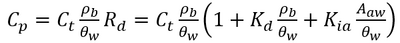
PFAS are a broad class of chemicals with highly variable chemical structures[24][25][26]. One characteristic feature of PFAS is that they are fluorosurfactants, distinct from more traditional hydrocarbon surfactants[25][27][28][29]. Fluorosurfactants typically have a fully or partially fluorinated, hydrophobic tail with ionic (cationic, zwitterionic, or anionic) head group that is hydrophilic[25][26]. The hydrophobic tail and ionic head group mean PFAS are very stable at hydrophobic adsorption interfaces when present in the aqueous phase[30]. Examples of these interfaces include naturally occurring organic matter in soils and the air-water interface in the vadose zone[31][32][33][34][35]. Their strong adsorption to both soil organic matter and the air-water interface is a major contributor to elevated concentrations of PFAS observed in the upper 5 feet of the soil column[19][20]. While several other PFAS partitioning processes exist[27], adsorption to solid phase soils and air-water interfaces are the two primary processes present at nearly all PFAS sites[36]. The total PFAS mass obtained from a vadose zone soil sample contains the solid phase, air-water interfacial, and aqueous phase PFAS mass, which can be converted to porewater concentrations using Equation 1[2].

Equation 1:   StultsEq1.png

Where Cp is the porewater concentration, Ct is the total PFAS concentration, ρb is the bulk density of the soil, θw is the volumetric water content, Rd is the PFAS retardation factor, Kd is the solid phase adsorption coefficient, Kia is the air-water interfacial adsorption coefficient, and Aaw is the air-water interfacial area. The air-water interfacial area of the soil is primarily a function of both the soil properties and the degree of volumetric water saturation in the soil. There are several methods of estimating air-water interfacial areas including thermodynamic functions based on the soil moisture retention curve. However, the thermodynamic function has been shown to underestimate air-water interfacial area[37], and must typically be scaled using empirical scaling factors. An empirical method recently developed to estimate air-water interfacial area is presented in Equation 2[37].

Equation 2:   StultsEq2.png

Where Sw is the water phase saturation as a ratio of the water content over the volumetric soil porosity, and d50 is the median grain diameter.

Lysimeters Background

Figure 1. (a) A field suction lysimeter with labeled parts typically used in field settings – Credit: Bibek Acharya and Dr. Vivek Sharma, UF/IFAS, https://edis.ifas.ufl.edu/publication/AE581. (b) Laboratory suction lysimeters used in Schaefer et al. 2024[5], which employed the use of micro-sampling suction lysimeters. (c) A field lysimeter used in Schaefer et al. 2023[16]. (d) Diagram of a drainage wicking lysimeter – Credit: Edaphic Scientific, https://edaphic.com.au/products/water/lysimeter-wick-for-drainage/

Lysimeters, generally speaking, refer to instruments which collect water from unsaturated soils[4][11]. However, there are multiple types of lysimeters which can be employed in field or laboratory settings. There are three primary types of lysimeters relevant to PFAS listed here and shown in Figure 1a-d.

  1. Suction Lysimeters (Figure 1a,b): These lysimeters are the most relevant for PFAS sampling and are the majority of discussion in this article. These lysimeters operate by extracting liquid from the unsaturated vadose zone by applying negative suction pressure at the sampling head[3][5][18]. The sampling head is typically constructed of porous ceramic or stainless steel. A PVC case or stainless-steel case is attached to the sampling head and extends upward above the ground surface. Suction lysimeters are typically installed between 1 and 9 feet below ground surface, but can extend as deep as 40-60 feet in some cases[3]. Shallow lysimeters (< 10 feet) are typically installed using a hand auger. For ceramic lysimeters, a silica flour slurry should be placed at the base of the bore hole and allowed to cover the ceramic head before backfilling the hole partially with natural soil. Once the hole is partially backfilled with soil to cover the sampling head, the remainder of the casing should be sealed with hydrated bentonite chips. When sampling events occur, suction is applied at the ground surface using a rubber gasket seal and a hand pump or electric pump. After sufficient porewater is collected (the time for which can vary greatly based on the soil permeability and moisture content), the seal can be removed and a peristaltic pump used to extract liquid from the lysimeter.
  2. Field Lysimeters (Figure 1c): These large lysimeters can be constructed from plastic or metal sidings. They can range from approximately 2 feet in diameter to as large as several meters in diameter[4]. Instrumentation such as soil moisture probes and tensiometers, or even multiple suction lysimeters, are typically placed throughout the lysimeter to measure the movement of water and determine characteristic soil moisture release curves[13][14][16][17][38]. Water is typically collected at the base of the field lysimeter to determine net recharge through the system. These field lysimeters are intended to represent more realistic, intermediate scale conditions of field systems.
  3. Drainage Lysimeters (Figure 1d): Also known as a “wick” lysimeter, these lysimeters typically consist of a hollow cup attached to a spout which protrudes above ground to relieve air pressure from the system and act as a sampling port. The hollow cup typically has filters and wicking devices at the base to collect water from the soil. The cup is filled with natural soil and collects water as it percolates through the vadose zone. These lysimeters are used to directly monitor net recharge from the vadose zone to the groundwater table and could be useful in determining PFAS mass flux.

Analysis of PFAS Concentrations in Soil and Porewater

Table 1. Measured and Predicted PFAS Concentrations in Porewater for Select PFAS in Three Different Soils
Site PFAS Field
Porewater
Concentration
(μg/L)
Lab Core
Porewater
Concentration
(μg/L)
Predicted
Porewater
Concentration
(μg/L)
Site A PFOS 6.2 ± 3.4 3.0 ± 0.37 6.6 ± 3.3
Site B PFOS 2.2 ± 2.0 0.78 ± 0.38 2.8
Site C PFOS 13 ± 4.1 680 ± 460 164 ± 75
8:2 FTS 1.2 ± 0.46 52 ± 13 16 ± 6.0
PFHpS 0.36 ± 0.051 2.9 ± 2.0 5.9 ± 3.4
Figure 2. Field Measured PFAS concentration Data (Orange) and Lab Core Measured Concentration Data (Blue) for four PFAS impacted sites[1]
Figure 3. Measured and predicted data for PFAS concentrations from a single site field lysimeter study. Model predictions both with and without PFAS sorption to the air-water interface were considered[16].

Schaefer et al.[5] measured PFAS porewater concentrations with field and laboratory suction lysimeters across several sites. Intact cores from the site were collected for soil water extraction using laboratory lysimeters. The lysimeters were used to directly compare field derived measurements of PFAS concentration in the mobile porewater phase. Results from measurements are for four sites presented in Figure 2.

Data from sites A and B showed reasonably good agreement (within ½ order of magnitude) for most PFAS measured in the systems. At site C, more hydrophobic constituents (> C6 PFAS) tended to have higher concentrations in the lab core than the field site while less hydrophobic constituents (< C6) had higher concentrations in the field than lab cores. Site D showed substantially greater (1 order of magnitude or more) PFAS concentrations measured in the laboratory-collected porewater sample compared to what was measured in the field lysimeters. This discrepancy for the Site D soil can likely be attributed to soil heterogeneity (as indicated by ground penetrating radar) and the fact that the soil consisted of back-filled materials rather than undisturbed native soils.

Site C showed elevated PFAS concentrations in the laboratory collected porewater for the more surface-active compounds. This increase was attributed to the soil wetting that occurred at the bench scale, which was reasonably described by the model shown in Equations 1 and 2 (see Table 1[1]). Equations 1 and 2 were also used to predict PFAS porewater concentrations (using porous cup lysimeters) in a highly instrumented test cell[16](Figure 3). The ability to predict soil concentrations from recurring porewater samples is critical to the practical application of lysimeters in field settings[1].

Results from suction lysimeters studies and field lysimeter studies show that PFAS concentrations in porewater predicted from soil concentrations using Equations 1 and 2 generally have reasonable agreement with measured in situ porewater data when air-water interfacial partitioning is considered. Results show that for less hydrophobic components like PFOA, the impact of air-water interfacial adsorption is less significant than for highly hydrophobic components like PFOS. The soil for the field lysimeter in Figure 3 was a sandy soil with a relatively low air-water interfacial area. The effect of air-water interfacial partitioning is expected to be much more significant for a greater range of PFAS in soils with high capillary pressure (i.e. silts/clays) with higher associated air-water interfacial areas[37][39][40].

Summary and Recommendations

The majority of research with lysimeters for PFAS site investigations has been done using porous cup suction lysimeters[3][1][5][18]. Porous cup suction lysimeters are advantageous because they can be routinely sampled or sampled after specific wetting or drying events much like groundwater wells. This sampling is easier and more efficient than routinely collecting soil samples from the same locations. Co-locating lysimeters with soil samples is important for establishing the baseline soil concentration levels at the lysimeter location and developing correlations between the soil concentrations and the mobile porewater concentration[3]. Appropriate standard operation procedures for lysimeter installation and operation have been established and have been reviewed in recent literature[3][5]. Lysimeters should typically be installed near the source area and just above the maximum groundwater level elevation to obtain accurate results of porewater concentrations year round. Depending upon the geology and vertical PFAS distribution in the soil, multilevel lysimeter installations should also be considered.

Results from several lysimeters studies across multiple field sites and modelling analysis has shown that lysimeters can produce reasonable results between field and laboratory studies[5][16][17]. Transient effects of wetting and drying as well as media heterogeneity affects appear to be responsible for some variability and uncertainty in lysimeter based PFAS measurements in the vadose zone. These mobile porewater concentrations can be coupled with effective recharge estimates and simplified modelling approaches to determine mass flux from the vadose zone to the underlying groundwater[15][22][2][41][42].

Future research opportunities should address the current key uncertainties related to the use of lysimeters for PFAS investigations, including:

  1. Collect larger datasets of PFAS concentrations to determine how transient wetting or drying periods and media type affect PFAS concentrations in the mobile porewater. Some research has shown that non-equilibrium processes can occur in the vadose zone, which can affect grab sample concentration in the porewater at specific time periods.
  2. More work should be done with flux averaging lysimeters like the drainage cup or wicking lysimeter. These lysimeters can directly measure net recharge and provide time averaged concentrations of PFAS in water over the sampling period. However, there is little work detailing their potential applications in PFAS research, or operational considerations for their use in remedial investigations for PFAS.
  3. Lysimeters should be coupled with monitoring of wetting and drying in the vadose zone using in situ soil moisture sensors or tensiometers and groundwater levels. Direct measurements of soil saturation at field sites are vital to directly correlate porewater concentrations with soil concentrations. Similarly, groundwater level fluctuations can inform net recharge estimates. By collecting these data we can continue to improve partitioning and leaching models which can relate porewater concentrations to total PFAS mass in soils and PFAS leaching at field sites.
  4. Comparisons of various bench-scale leaching or desorption tests to field-based lysimeter data are recommended. The ability to correlate field measurements of PFAS concentrations with estimates of leaching from laboratory studies would provide a powerful method to empirically estimate PFAS leaching from field sites.

References

  1. ^ 1.0 1.1 1.2 1.3 1.4 1.5 1.6 Anderson, R.H., Feild, J.B., Dieffenbach-Carle, H., Elsharnouby, O., Krebs, R.K., 2022. Assessment of PFAS in Collocated Soil and Porewater Samples at an AFFF-Impacted Source Zone: Field-Scale Validation of Suction Lysimeters. Chemosphere, 308(1), Article 136247. doi: 10.1016/j.chemosphere.2022.136247
  2. ^ 2.0 2.1 2.2 2.3 Brusseau, M.L., Guo, B., 2022. PFAS Concentrations in Soil versus Soil Porewater: Mass Distributions and the Impact of Adsorption at Air-Water Interfaces. Chemosphere, 302, Article 134938. doi: 10.1016/j.chemosphere.2022.134938  Open Access Manuscript
  3. ^ 3.0 3.1 3.2 3.3 3.4 3.5 3.6 Costanza, J., Clabaugh, C.D., Leibli, C., Ferreira, J., Wilkin, R.T., 2025. Using Suction Lysimeters for Determining the Potential of Per- and Polyfluoroalkyl Substances to Leach from Soil to Groundwater: A Review. Environmental Science and Technology, 59(9), pp. 4215-4229. doi: 10.1021/acs.est.4c10246
  4. ^ 4.0 4.1 4.2 4.3 Meissner, R., Rupp, H., Haselow, L., 2020. Use of Lysimeters for Monitoring Soil Water Balance Parameters and Nutrient Leaching. In: Climate Change and Soil Interactions. Elsevier, pp. 171-205. doi: 10.1016/B978-0-12-818032-7.00007-2
  5. ^ 5.0 5.1 5.2 5.3 5.4 5.5 5.6 5.7 Schaefer, C.E., Nguyen, D., Fang, Y., Gonda, N., Zhang, C., Shea, S., Higgins, C.P., 2024. PFAS Porewater Concentrations in Unsaturated Soil: Field and Laboratory Comparisons Inform on PFAS Accumulation at Air-Water Interfaces. Journal of Contaminant Hydrology, 264, Article 104359. doi: 10.1016/j.jconhyd.2024.104359  Open Access Manuscript
  6. ^ 6.0 6.1 Goss, M.J., Ehlers, W., 2009. The Role of Lysimeters in the Development of Our Understanding of Soil Water and Nutrient Dynamics in Ecosystems. Soil Use and Management, 25(3), pp. 213–223. doi: 10.1111/j.1475-2743.2009.00230.x
  7. ^ Pütz, T., Fank, J., Flury, M., 2018. Lysimeters in Vadose Zone Research. Vadose Zone Journal, 17 (1), pp. 1-4. doi: 10.2136/vzj2018.02.0035  Open Access Article
  8. ^ Bergström, L., 1990. Use of Lysimeters to Estimate Leaching of Pesticides in Agricultural Soils. Environmental Pollution, 67 (4), 325–347. doi: 10.1016/0269-7491(90)90070-S
  9. ^ Dabrowska, D., Rykala, W., 2021. A Review of Lysimeter Experiments Carried Out on Municipal Landfill Waste. Toxics, 9(2), Article 26. doi: 10.3390/toxics9020026  Open Access Article
  10. ^ Fernando, S.U., Galagedara, L., Krishnapillai, M., Cuss, C.W., 2023. Lysimeter Sampling System for Optimal Determination of Trace Elements in Soil Solutions. Water, 15(18), Article 3277. doi: 10.3390/w15183277  Open Access Article
  11. ^ 11.0 11.1 Rogers, R.D., McConnell, J.W. Jr., 1993. Lysimeter Literature Review, Nuclear Regulatory Commission Report Numbers: NUREG/CR--6073, EGG--2706. [1] ID: 10183270. doi: 10.2172/10183270  Open Access Article
  12. ^ Sołtysiak, M., Rakoczy, M., 2019. An Overview of the Experimental Research Use of Lysimeters. Environmental and Socio-Economic Studies, 7(2), pp. 49-56. doi: 10.2478/environ-2019-0012  Open Access Article
  13. ^ 13.0 13.1 Stannard, D.I., 1992. Tensiometers—Theory, Construction, and Use. Geotechnical Testing Journal, 15(1), pp. 48-58. doi: 10.1520/GTJ10224J
  14. ^ 14.0 14.1 Winton, K., Weber, J.B., 1996. A Review of Field Lysimeter Studies to Describe the Environmental Fate of Pesticides. Weed Technology, 10(1), pp. 202-209. doi: 10.1017/S0890037X00045929
  15. ^ 15.0 15.1 15.2 Anderson, R.H., 2021. The Case for Direct Measures of Soil-to-Groundwater Contaminant Mass Discharge at AFFF-Impacted Sites. Environmental Science and Technology, 55(10), pp. 6580-6583. doi: 10.1021/acs.est.1c01543
  16. ^ 16.0 16.1 16.2 16.3 16.4 16.5 16.6 Schaefer, C.E., Lavorgna, G.M., Lippincott, D.R., Nguyen, D., Schaum, A., Higgins, C.P., Field, J., 2023. Leaching of Perfluoroalkyl Acids During Unsaturated Zone Flushing at a Field Site Impacted with Aqueous Film Forming Foam. Environmental Science and Technology, 57(5), pp. 1940-1948. doi: 10.1021/acs.est.2c06903
  17. ^ 17.0 17.1 17.2 Schaefer, C.E., Lavorgna, G.M., Lippincott, D.R., Nguyen, D., Christie, E., Shea, S., O’Hare, S., Lemes, M.C.S., Higgins, C.P., Field, J., 2022. A Field Study to Assess the Role of Air-Water Interfacial Sorption on PFAS Leaching in an AFFF Source Area. Journal of Contaminant Hydrology, 248, Article 104001. doi: 10.1016/j.jconhyd.2022.104001  Open Access Manuscript
  18. ^ 18.0 18.1 18.2 Quinnan, J., Rossi, M., Curry, P., Lupo, M., Miller, M., Korb, H., Orth, C., Hasbrouck, K., 2021. Application of PFAS-Mobile Lab to Support Adaptive Characterization and Flux-Based Conceptual Site Models at AFFF Releases. Remediation, 31(3), pp. 7-26. doi: 10.1002/rem.21680
  19. ^ 19.0 19.1 Brusseau, M.L., Anderson, R.H., Guo, B., 2020. PFAS Concentrations in Soils: Background Levels versus Contaminated Sites. Science of The Total Environment, 740, Article 140017. doi: 10.1016/j.scitotenv.2020.140017
  20. ^ 20.0 20.1 Bigler, M.C., Brusseau, M.L., Guo, B., Jones, S.L., Pritchard, J.C., Higgins, C.P., Hatton, J., 2024. High-Resolution Depth-Discrete Analysis of PFAS Distribution and Leaching for a Vadose-Zone Source at an AFFF-Impacted Site. Environmental Science and Technology, 58(22), pp. 9863-9874. doi: 10.1021/acs.est.4c01615
  21. ^ Nickerson, A., Maizel, A.C., Kulkarni, P.R., Adamson, D.T., Kornuc, J. J., Higgins, C.P., 2020. Enhanced Extraction of AFFF-Associated PFASs from Source Zone Soils. Environmental Science and Technology, 54(8), pp. 4952-4962. doi: 10.1021/acs.est.0c00792
  22. ^ 22.0 22.1 Stults, J.F., Schaefer, C.E., Fang, Y., Devon, J., Nguyen, D., Real, I., Hao, S., Guelfo, J.L., 2024. Air-Water Interfacial Collapse and Rate-Limited Solid Desorption Control Perfluoroalkyl Acid Leaching from the Vadose Zone. Journal of Contaminant Hydrology, 265, Article 104382. doi: 10.1016/j.jconhyd.2024.104382  Open Access Manuscript
  23. ^ Stults, J.F., Choi, Y.J., Rockwell, C., Schaefer, C.E., Nguyen, D.D., Knappe, D.R.U., Illangasekare, T.H., Higgins, C.P., 2023. Predicting Concentration- and Ionic-Strength-Dependent Air–Water Interfacial Partitioning Parameters of PFASs Using Quantitative Structure–Property Relationships (QSPRs). Environmental Science and Technology, 57(13), pp. 5203-5215. doi: 10.1021/acs.est.2c07316
  24. ^ Moody, C.A., Field, J.A., 1999. Determination of Perfluorocarboxylates in Groundwater Impacted by Fire-Fighting Activity. Environmental Science and Technology, 33(16), pp. 2800-2806. doi: 10.1021/es981355+
  25. ^ 25.0 25.1 25.2 Moody, C.A., Field, J.A., 2000. Perfluorinated Surfactants and the Environmental Implications of Their Use in Fire-Fighting Foams. Environmental Science and Technology, 34(18), pp. 3864-3870. doi: 10.1021/es991359u
  26. ^ 26.0 26.1 Glüge, J., Scheringer, M., Cousins, I.T., DeWitt, J.C., Goldenman, G., Herzke, D., Lohmann, R., Ng, C.A., Trier, X., Wang, Z., 2020. An Overview of the Uses of Per- and Polyfluoroalkyl Substances (PFAS). Environmental Science: Processes and Impacts, 22(12), pp. 2345-2373. doi: 10.1039/D0EM00291G  Open Access Article
  27. ^ 27.0 27.1 Brusseau, M.L., 2018. Assessing the Potential Contributions of Additional Retention Processes to PFAS Retardation in the Subsurface. Science of The Total Environment, 613-614, pp. 176-185. doi: 10.1016/j.scitotenv.2017.09.065  Open Access Manuscript
  28. ^ Dave, N., Joshi, T., 2017. A Concise Review on Surfactants and Its Significance. International Journal of Applied Chemistry, 13(3), pp. 663-672. doi: 10.37622/IJAC/13.3.2017.663-672  Open Access Article
  29. ^ García, R.A., Chiaia-Hernández, A.C., Lara-Martin, P.A., Loos, M., Hollender, J., Oetjen, K., Higgins, C.P., Field, J.A., 2019. Suspect Screening of Hydrocarbon Surfactants in Afffs and Afff-Contaminated Groundwater by High-Resolution Mass Spectrometry. Environmental Science and Technology, 53(14), pp. 8068-8077. doi: 10.1021/acs.est.9b01895
  30. ^ Krafft, M.P., Riess, J.G., 2015. Per- and Polyfluorinated Substances (PFASs): Environmental Challenges. Current Opinion in Colloid and Interface Science, 20(3), pp. 192-212. doi: 10.1016/j.cocis.2015.07.004
  31. ^ Schaefer, C.E., Culina, V., Nguyen, D., Field, J., 2019. Uptake of Poly- and Perfluoroalkyl Substances at the Air–Water Interface. Environmental Science and Technology, 53(21), pp. 12442-12448. doi: 10.1021/acs.est.9b04008
  32. ^ Lyu, Y., Brusseau, M.L., Chen, W., Yan, N., Fu, X., Lin, X., 2018. Adsorption of PFOA at the Air–Water Interface during Transport in Unsaturated Porous Media. Environmental Science and Technology, 52(14), pp. 7745-7753. doi: 10.1021/acs.est.8b02348
  33. ^ Costanza, J., Arshadi, M., Abriola, L.M., Pennell, K.D., 2019. Accumulation of PFOA and PFOS at the Air-Water Interface. Environmental Science and Technology Letters, 6(8), pp. 487-491. doi: 10.1021/acs.estlett.9b00355
  34. ^ Li, F., Fang, X., Zhou, Z., Liao, X., Zou, J., Yuan, B., Sun, W., 2019. Adsorption of Perfluorinated Acids onto Soils: Kinetics, Isotherms, and Influences of Soil Properties. Science of The Total Environment, 649, pp. 504-514. doi: 10.1016/j.scitotenv.2018.08.209
  35. ^ Nguyen, T.M.H., Bräunig, J., Thompson, K., Thompson, J., Kabiri, S., Navarro, D.A., Kookana, R.S., Grimison, C., Barnes, C.M., Higgins, C.P., McLaughlin, M.J., Mueller, J.F., 2020. Influences of Chemical Properties, Soil Properties, and Solution pH on Soil–Water Partitioning Coefficients of Per- and Polyfluoroalkyl Substances (PFASs). Environmental Science and Technology, 54(24), pp. 15883-15892. doi: 10.1021/acs.est.0c05705  Open Access Article
  36. ^ Brusseau, M.L., Yan, N., Van Glubt, S., Wang, Y., Chen, W., Lyu, Y., Dungan, B., Carroll, K.C., Holguin, F.O., 2019. Comprehensive Retention Model for PFAS Transport in Subsurface Systems. Water Research, 148, pp. 41-50. doi: 10.1016/j.watres.2018.10.035
  37. ^ 37.0 37.1 37.2 Brusseau, M.L., 2023. Determining Air-Water Interfacial Areas for the Retention and Transport of PFAS and Other Interfacially Active Solutes in Unsaturated Porous Media. Science of The Total Environment, 884, Article 163730. doi: 10.1016/j.scitotenv.2023.163730  Open Access Article
  38. ^ van Genuchten, M.Th. , 1980. A Closed‐form Equation for Predicting the Hydraulic Conductivity of Unsaturated Soils. Soil Science Society of America Journal, 44(5), pp. 892-898. doi: 10.2136/sssaj1980.03615995004400050002x
  39. ^ Peng, S., Brusseau, M.L., 2012. Air-Water Interfacial Area and Capillary Pressure: Porous-Medium Texture Effects and an Empirical Function. Journal of Hydrologic Engineering, 17(7), pp. 829-832. doi: 10.1061/(asce)he.1943-5584.0000515
  40. ^ Brusseau, M.L., Peng, S., Schnaar, G., Costanza-Robinson, M.S., 2006. Relationships among Air-Water Interfacial Area, Capillary Pressure, and Water Saturation for a Sandy Porous Medium. Water Resources Research, 42(3), Article W03501, 5 pages. doi: 10.1029/2005WR004058  Free Access Article
  41. ^ Stults, J.F., Schaefer, C.E., MacBeth, T., Fang, Y., Devon, J., Real, I., Liu, F., Kosson, D., Guelfo, J.L., 2025. Laboratory Validation of a Simplified Model for Estimating Equilibrium PFAS Mass Leaching from Unsaturated Soils. Science of The Total Environment, 970, Article 179036. doi: 10.1016/j.scitotenv.2025.179036
  42. ^ Smith, J. Brusseau, M.L., Guo, B., 2024. An Integrated Analytical Modeling Framework for Determining Site-Specific Soil Screening Levels for PFAS. Water Research, 252, Article121236. doi: 10.1016/j.watres.2024.121236

See Also